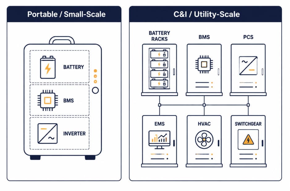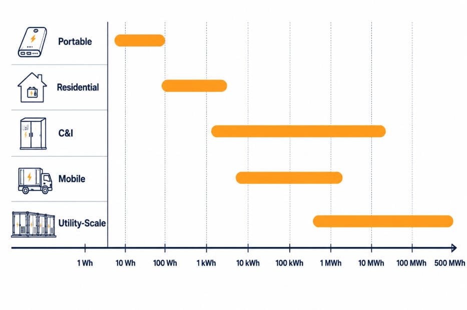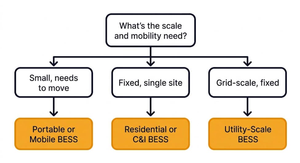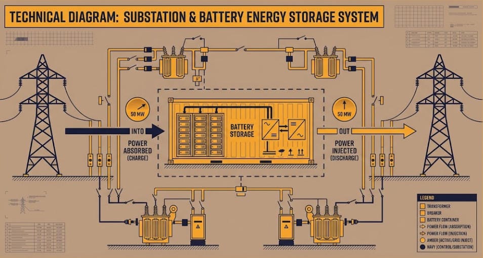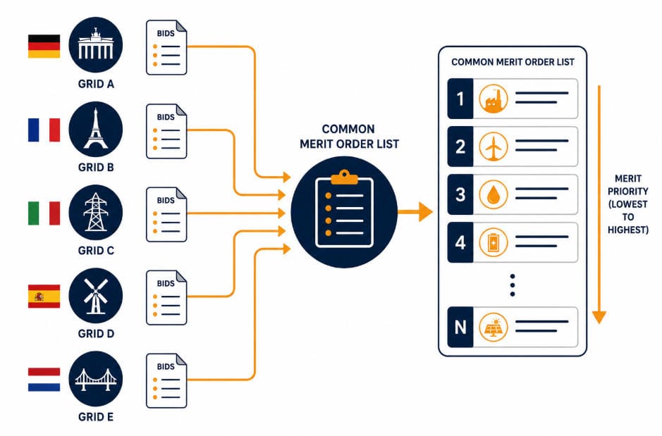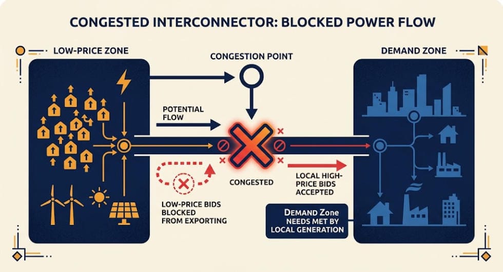
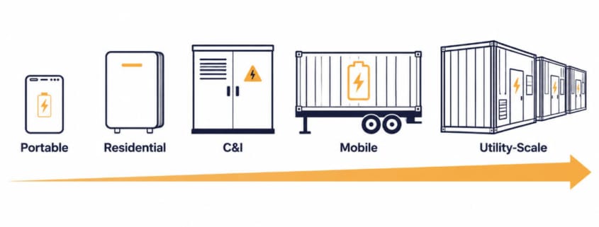
C&I vs utility-scale is the first question every solar or battery storage project must answer. The two terms sound like simple size labels. In reality, they describe two very different businesses. Not only do they serve different customers, but they also connect to the grid differently and rely on entirely unique financing and equipment. This guide walks through the full C&I vs utility-scale comparison, section by section, so you know exactly which one applies to your project.
⚡ Quick Answer: C&I vs Utility-Scale In short, C&I vs utility-scale comes down to one factor: what sits behind the grid connection. A C&I system serves a single business site and lowers that site’s own electricity bill. A utility-scale system, on the other hand, connects straight to the grid and sells power to the wider market. Everything else — size, financing, interconnection, and equipment — follows from that one distinction.
C&I vs Utility-Scale: Key Differences at a Glance
Before the full breakdown, here’s the short version of the comparison:
Size: C&I typically runs 100 kW to 10 MW. Utility-scale typically runs 20 MW to 500+ MW.
Connection: C&I sits behind the meter. Utility-scale sits in front of it.
Revenue: C&I saves money on one facility’s bill. Utility-scale earns revenue from the wholesale market.
Timeline: C&I projects often finish in months. Utility-scale projects often take years.
Ownership: hosts or third-party lessors typically own C&I systems. Independent power producers typically own utility-scale plants.
What Does C&I Mean?
C&I stands for Commercial and Industrial. In the BESS world, it describes systems installed at a business’s own site. Picture a factory, a warehouse, a distribution center, or a hospital. These systems serve that facility’s own electricity needs. Specifically, C&I systems typically range from 100 kW to a few megawatts (MW). Large industrial campuses can reach 5–10 MW.
A C&I system sits behind the customer’s meter. Its main job is cutting that facility’s electricity bill, not selling power onto the grid. For that reason, businesses deploy C&I storage for several reasons:
Demand charge reduction — the battery discharges during peak demand and shaves the facility’s peak draw. Utilities bill demand separately from energy, often heavily. As a result, peak shaving delivers one of the fastest paybacks in the industry.
Time-of-use (TOU) arbitrage — the system charges when electricity is cheap and discharges when it’s expensive.
Backup power — stored energy keeps critical loads running through an outage.
Solar self-consumption — pairing storage with on-site solar lets the facility use more of its own generation instead of exporting it.
Demand response — the facility earns payments for cutting load when asked.
In addition, every one of these applications runs on the same core hardware — batteries, inverters, and enclosures — covered in our guide to the key components of a C&I BESS.
What Does Utility-Scale Mean?
Utility-scale storage means large power plants. Some call it grid-scale or front-of-the-meter storage. These plants typically run from tens of megawatts to several hundred megawatts. The largest projects reach the gigawatt range for total energy capacity. Unlike C&I systems, utility-scale plants don’t serve one building. Instead, they connect directly to the transmission grid or a high-voltage line, and they sell power and grid services into the wholesale market.
Developers build, own, and operate these projects as standalone power plants. Revenue comes from several sources:
Power purchase agreements (PPAs) with a utility or corporate offtaker
Wholesale energy market sales — buying low and selling high across the day
Ancillary services, such as frequency regulation, spinning reserve, and capacity payments
Resource adequacy and capacity markets, which pay the plant to stay available during system peaks
Most people reach for size first when they compare C&I vs utility-scale projects. But size is only a side effect, not the real distinction. The true dividing line is simpler: does an existing load sit behind the grid connection?
A C&I plant connects at a site with an existing load — a factory, a data center, a logistics hub — and the battery interacts with that load. A utility-scale plant, by contrast, connects at a site built only for the plant itself. No meaningful load sits behind it. The plant exists purely to generate or store energy for the grid.
This explains an unusual case. A data center with tens of megawatt-hours of storage still counts as C&I, because a load sits behind the meter. A small dedicated battery plant on a remote substation still counts as utility-scale, because no load does. In short, size alone never decides the category.
C&I vs Utility-Scale: Side-by-Side Comparison
The table below summarizes the core C&I vs utility-scale differences at a glance.
Attribute
C&I
Utility-Scale
Typical size
~100 kW – 10 MW
~20 MW – 500+ MW
Connection point
Behind the customer’s meter, low/medium voltage
Front-of-the-meter, transmission or sub-transmission voltage
Primary customer
The host facility (factory, warehouse, campus)
The grid / wholesale market / utility offtaker
Main value streams
Demand charge reduction, TOU arbitrage, backup power, self-consumption
Energy arbitrage, capacity payments, ancillary services, PPA revenue
Ownership model
Facility owner, third-party PPA/lease, or ESA
Independent power producer (IPP), utility, or institutional investor
Site control
Existing commercial/industrial property
Purpose-acquired land, often rural
Interconnection process
Utility’s commercial/small-generator process
RTO/ISO or utility large-generator interconnection queue
Typical BESS duration
1–4 hours
2–8+ hours, growing interest in long-duration storage
Design driver
Facility load profile and tariff structure
Market price signals and grid needs
Permitting complexity
Lower — usually local/municipal
Higher — environmental review, land use, transmission studies
Typical project timeline
Months
Multiple years, often 3–7 years including interconnection queue
Typical payback / horizon
3–7 years, driven by demand charges and tariff spreads
10–15+ years, underwritten by long-term PPA and market revenue
C&I vs Utility-Scale: Technical Differences
Size and connection point drive real engineering differences between C&I vs utility-scale systems. Here’s how they show up in practice, category by category.
Voltage and Interconnection Equipment
C&I systems usually interconnect at low voltage (400–480V) or medium voltage (4.16–34.5 kV). They tie directly into a building’s electrical service or a nearby feeder. Utility-scale systems, however, interconnect at transmission-class voltages, often 69 kV and above. That higher voltage requires dedicated substations, step-up transformers, and compliance with the utility’s or ISO’s large-generator interconnection agreement.
Control and Dispatch Strategy
A C&I energy management system (EMS) tunes itself around the host facility’s own load curve. Specifically, it tracks peak demand windows and the site’s utility tariff. A utility-scale EMS, in contrast, tunes around market price signals and grid-operator dispatch instructions. Increasingly, it also stacks multiple revenue streams at once — a practice the industry calls value stacking.
Duration, Cycling, and Modularity
C&I batteries commonly run 1–4 hour discharge durations, matched to typical demand-charge windows. Utility-scale batteries, meanwhile, increasingly target longer durations — 4, 8, or more hours — to cover evening peaks as solar output fades. As a result, they also cycle more predictably against known market patterns.
Physical layout differs too. C&I deployments often use a few large enclosures sized to fit an existing footprint, such as a rooftop or a parking area. Utility-scale projects, by comparison, deploy dozens to hundreds of containerized units across open land, in a standardized layout built for construction speed.
Inverter Control Mode
Roughly 80–85% of all BESS installed worldwide today use grid-following (GFL) inverters, which lock onto an existing grid signal. Utility-scale projects, however, increasingly specify grid-forming (GFM) inverters instead. These can lightweight-synthesize their own voltage and frequency reference, support black start, and provide synthetic inertia.
While those capabilities matter far more at grid scale than behind a single facility’s meter, there is a major exception emerging in the C&I space: advanced microgrids. High-reliability C&I applications—such as islanded critical infrastructure, data centers, or remote mining sites—are actively adopting grid-forming inverters. This allows the facility to safely intentional-island from the main grid during an outage and maintain seamless, resilient operations on its own terms.
Codes and Standards
Both categories follow UL 9540 for energy storage systems, UL 9540A for thermal runaway fire testing, and NFPA 855, the primary U.S. fire code for stationary energy storage. or a deep dive into the latest safety rules, spacing requirements, and hazard testing under this framework, read our comprehensive NFPA 855 guide.
Utility-scale sites, however, carry extra requirements tied to grid interconnection standards. Examples include IEEE 1547 for distributed resources and FERC/NERC reliability rules for transmission-connected assets. C&I systems, meanwhile, must satisfy local fire marshal and building code review, since they sit next to occupied buildings.
C&I vs Utility-Scale Interconnection Process
Interconnection turns the C&I vs utility-scale comparison into a real scheduling and risk problem, not just an engineering one.
C&I Interconnection
A C&I system typically goes through the utility’s existing commercial or small-generator interconnection process. Because the site already connects to the grid, the project doesn’t need new transmission infrastructure. As a result, timelines usually run from a few weeks to a few months.
Utility-Scale Interconnection
A utility-scale project must apply to the regional transmission organization (RTO) or independent system operator (ISO), or to the relevant utility, through a large-generator interconnection queue. FERC sets the federal rules for this process, which includes system impact studies and facilities studies. It often requires the developer to fund network upgrades the studies identify.
Interconnection queues in many U.S. regions now run 3–5+ years. Some run much longer. Because of this, interconnection timing is one of the biggest risk factors in utility-scale project development.
C&I vs Utility-Scale: Financing and Economics
C&I projects usually rely on financing built for a single host customer. A business might pay cash, sign a storage lease, or use a third-party-owned power purchase agreement, where a developer owns the system and the host simply pays for the savings it delivers. Payback typically lands in the 3–7 year range, depending on local demand-charge structure. For the full ROI math, see our guide to C&I BESS economics.
Utility-scale projects, by contrast, raise money as standalone infrastructure assets. Developers combine tax equity, debt from infrastructure lenders, and a long-term PPA that underwrites the debt. Because no single host’s bill defines success, the economics depend on wholesale market forecasts and interconnection terms. Investment horizons commonly run 10–15+ years. For the full framework on calculating storage ROI, see our guide to the economics of BESS.
Permitting complexity follows the same pattern. C&I projects mainly clear local and municipal review. Utility-scale projects, however, add environmental review, land-use approval, and formal interconnection studies on top.
C&I vs Utility-Scale: Which One Fits Your Project?
The right category isn’t really a choice. It follows from the problem you’re solving.
If the goal is to lower one facility’s bill, add resiliency, or manage demand charges, C&I is the answer — sized and controlled around that facility’s own load and tariff.
If the goal is to earn revenue by selling power or grid services into the wholesale market, utility-scale is the answer — sited and interconnected as a standalone power plant.
Some organizations pursue both. For example, a large industrial company might install a C&I system at its own plant while also investing in a utility-scale project as a corporate PPA offtaker. Either way, the two remain distinct engineering and financial exercises, even inside the same company.
Key Takeaways: C&I vs Utility-Scale The C&I vs utility-scale decision starts with one question: is there a load behind the meter? If yes, the project is C&I. If no, it’s utility-scale. Everything else — voltage, control strategy, financing, and interconnection — follows from that single fact.Sunlith Energy reviews incoming cell test data, matching tolerances, and pack assembly quality control for BESS projects from 50 kWh upward. Contact us before you finalize a cell or pack supplier.
C&I vs Utility-Scale FAQs
Is a community solar project C&I or utility-scale?
Community solar projects behave more like small utility-scale assets. They interconnect to the distribution grid and sell subscriptions, rather than serving one host’s load. That said, they’re usually smaller — 1–5 MW — than a traditional utility-scale plant.
Can a C&I battery ever sell power back to the grid?
Some C&I systems do join demand response or limited export programs. Even so, their main job stays the same: cut the host facility’s own costs. That’s what separates them from front-of-the-meter assets built mainly to sell power.
Does utility-scale mean the utility owns it?
Not necessarily. Independent power producers and investment funds own many utility-scale plants. They simply sell power to a utility or corporate buyer under a PPA. In other words, the term describes the scale and grid connection point, not the owner.
Why do C&I projects move faster than utility-scale projects?
C&I systems interconnect at lower voltage through a simpler utility process. They usually skip new transmission infrastructure entirely. As a result, they avoid the multi-year interconnection queues that utility-scale projects face at the transmission level.
Is project size or the meter connection the real dividing line?
The meter connection decides it. A large facility with tens of megawatt-hours of storage still counts as C&I, because a load sits behind the connection. A small dedicated battery plant on a remote substation still counts as utility-scale, because no load does.
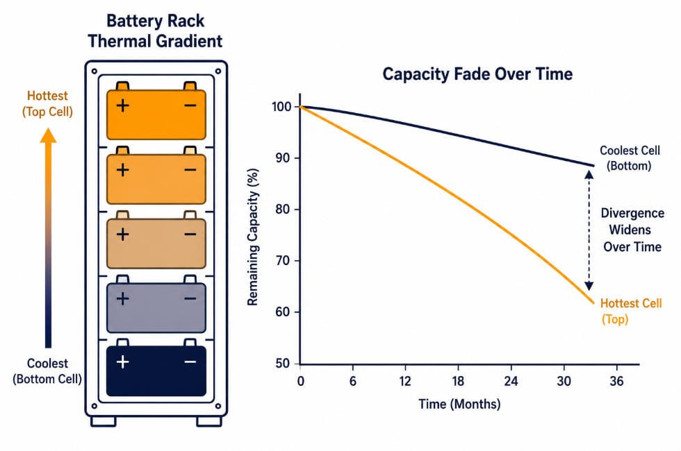
⚡ Quick Answer: What Is a Safe Temperature Gradient in a BESS Pack? A temperature gradient is the difference in temperature between the hottest and coolest cells in a pack at the same moment, often written as ΔT. Many BESS specifications target a maximum gradient of around 5°C across a rack, with premium liquid-cooled systems aiming closer to 2-3°C. A larger temperature gradient does not just mean one hot spot. It means cells are aging at different rates within the same pack, which widens the performance gap that cell matching worked to close in the first place.
1. Why Temperature Uniformity Is a Different Problem Than Cooling Capacity
Choosing between air and liquid cooling answers one question: how much heat can the system remove overall. It does not answer a second, separate question, however: does that heat leave every cell at the same rate? A BESS can have more than enough total cooling capacity. Even so, it can still run a large temperature gradient, if heat leaves some cells faster than others.
This distinction matters because gradient problems do not always show up as an overheating alarm. A pack can sit comfortably within its overall safe temperature range. Meanwhile, one corner of the rack quietly runs several degrees hotter than another, cycle after cycle. Nothing trips. Nothing alarms. The pack simply ages unevenly, and nobody notices until the SOH numbers start to diverge.
2. What Counts as a Safe Temperature Gradient
Exact gradient limits vary by manufacturer, cell chemistry, and system design. As a result, treat any single number as a target to verify, not a universal rule. That said, a few reference points are commonly cited in BESS specifications.
Around 5°C maximum cell-to-cell gradient is a commonly specified ceiling for air-cooled and moderately cooled BESS racks.
2-3°C is a tighter target that premium liquid-cooled systems often aim for, particularly at utility scale, where thousands of cells raise the stakes of even small mismatches.
Gradient limits typically apply within a single rack or module first. They then get checked again at the full-system level, since gradients between racks can run larger than gradients within one rack.
Ask your supplier for their specific gradient target, not just their overall operating temperature range. A wide operating range, such as -20°C to 55°C, says nothing about how tightly matched cell temperatures stay relative to each other inside that range.
3. Three Root Causes of Uneven Cell Heating
Temperature gradients rarely come from one single cause. Instead, three factors typically combine to create them.
Coolant Path Position
In a liquid-cooled rack, coolant usually enters at one point and exits at another, picking up heat along the way. Cells nearest the coolant inlet sit in cooler fluid. Cells nearest the outlet, by contrast, sit in fluid that has already absorbed heat from cells earlier in the path. As a result, outlet-side cells often run measurably warmer than inlet-side cells. This happens purely because of their position in the flow path, not because of anything different about the cells themselves.
Cell Position Within the Pack
Cells near the edge of a rack or enclosure sit closer to the outside walls, where some heat escapes to the surrounding air. Cells buried in the center of a dense pack, on the other hand, have neighbors on every side, so that heat has fewer places to go. Center cells, therefore, often run hotter than edge cells, even under identical cooling and identical current.
Current Path and Busbar Resistance
Current does not always split perfectly evenly across parallel cell groups. Small differences in busbar length, connection quality, or contact resistance mean some current paths carry slightly more current than others. Since heating from resistance follows I²R, even a small current imbalance produces a disproportionate heating difference. This connects directly to internal resistance variation covered in our cell matching guide: cells or groups with higher resistance generate more heat at the same current. As a result, a resistance mismatch and a temperature gradient often reinforce each other.
4. How a Temperature Gradient Accelerates Divergent Aging
Battery aging reactions speed up with heat. Researchers publishing in PMC (National Center for Biotechnology Information) found that inhomogeneous cell temperature inside a pack is a real, measurable driver of uneven degradation, not just a theoretical concern. Applied to a pack with a real gradient, this means the hottest cells are not just uncomfortable. They are quietly aging faster than their cooler neighbors, cycle after cycle.
This is where uneven heating and cell matching intersect. A pack that started out well matched, as covered in our cell matching guide, can still drift apart over time. A persistent hot zone can push those cells toward faster capacity fade. Meanwhile, cooler cells barely age at all. The BMS then has to work harder to compensate for a gap that thermal design, not manufacturing variance, actually created.
Cold cells create a different problem. Below their optimal range, cells deliver less power. They also accept slower charge rates. In practice, this means the coolest cells in a pack can become the limiting factor for dispatch power. This happens even though they are aging the slowest of anyone in the rack.
5. How the BMS Responds to What It Can Actually See
A BMS cannot manage a gradient it cannot measure. Sensor placement, therefore, matters as much as sensor accuracy. A design with one temperature sensor per module, placed at a single convenient point, will miss gradients happening between that sensor’s location and the rest of the module.
More thorough designs, instead, place multiple sensors per module. These sit at known high-risk points — near coolant outlets, at pack centers, and at busbar connections. This ties directly into the safety diagnostic algorithms covered in our BMS algorithms guide, since a BMS can only flag a developing hot spot if a sensor actually sits close enough to detect it before the gradient becomes a real problem.
6. Questions to Ask Your Supplier
What is your specified maximum cell-to-cell temperature gradient, not just the overall operating temperature range?
How many temperature sensors does each module have, and where are they physically placed?
For liquid-cooled systems, what is the coolant flow path? What gradient exists between inlet-side and outlet-side cells?
Do you have field or test data showing SOH divergence between hot-zone and cool-zone cells over time?
How does the BMS respond if a persistent gradient develops? Does it just log the data, or does it adjust balancing or dispatch limits?
Conclusion: A Temperature Gradient Is a Slow Problem That Looks Like No Problem at All
Overheating alarms are easy to notice. Temperature gradients, however, are not. A pack can run entirely within its safe range. It can still age unevenly, cell by cell. Nobody measured the gradient closely enough to see it. Ask suppliers for their specific gradient limit, not just their operating range. Then ask how many sensors actually watch for it.
For the manufacturing-stage half of this problem — how mismatched cells enter a pack in the first place — see our cell matching guide. Matching and thermal design solve two different sources of the same underlying issue: cells in one pack quietly drifting apart from each other over time.
☀️ Need a Thermal Design Review for Your BESS Project? Sunlith Energy reviews cooling architecture, sensor placement, and gradient specifications for BESS projects from 50 kWh upward. Contact us before you finalize a thermal design.
Frequently Asked Questions About Cell Temperature Gradients
What is a temperature gradient in a battery pack?
A temperature gradient is the difference between the hottest and coolest cell temperatures in a pack at the same moment, usually written as ΔT. It is a separate measurement from the pack’s overall operating temperature range. That is because a pack can sit within a safe range overall while still having a large gap between its warmest and coolest cells.
What causes temperature gradients inside a BESS pack?
Three factors typically combine to cause gradients. Coolant path position matters, since cells near a coolant outlet run warmer than cells near the inlet. Cell position within the pack matters too, since center cells trap more heat than edge cells. Finally, uneven current distribution from busbar resistance differences creates uneven I²R heating across parallel cell groups.
How does uneven heating affect cell aging?
Hotter cells within a gradient age faster than cooler cells in the same pack, since battery degradation reactions speed up with heat. Over time, this can widen the performance gap between cells, even in a pack that started out well matched. As a result, the BMS ends up compensating for a gap that thermal design created, rather than manufacturing variance.
What is a safe temperature gradient for a BESS pack?
Exact limits vary by manufacturer and system design. However, a maximum gradient of around 5°C is commonly specified for air-cooled and moderately cooled systems, while premium liquid-cooled systems often target 2-3°C. Always confirm the specific figure with your supplier rather than assuming a standard number applies.
How many temperature sensors does a BESS module need?
There is no single universal number. Still, a module with only one sensor at a single convenient location cannot detect a gradient occurring elsewhere in that module. More thorough designs, therefore, place multiple sensors at known high-risk points, such as near coolant outlets, pack centers, and busbar connections.
⚡ Quick Answer: Which BMS Architecture Is Right for a BESS? BMS architecture comes in three main types: centralised (one controller handles all cells directly), modular master-slave (each module has its own slave BMS reporting to a master), and wireless BMS (modules communicate without a physical data harness). Centralised suits small residential systems. Modular master-slave is the standard for commercial and utility-scale BESS. Wireless BMS is maturing fast in EVs but remains early-stage for grid-scale BESS, mainly due to EMI risk in high-power environments and a 25-40% cost premium.
1. Why BMS Architecture Matters Beyond Just System Size
Most guides treat BMS architecture as a simple size question: small systems get one BMS, big systems get many. That is true as a starting point. But the choice also decides how a fault in one module affects the rest of the pack, how much wiring a technician has to run and maintain, and how easily the system scales later without a redesign.
For the basics of what a BMS does — monitoring, protection, balancing, and communication — see our complete battery management system guide. This article goes one level deeper: the wiring topology inside modular designs, and the wireless BMS option now entering the market.
2. Centralised BMS: How a Single Controller Works
In a centralised design, one controller connects directly to every cell in the pack. It handles voltage monitoring, balancing, and protection for all cells from a single board. There is no master-slave hierarchy here, simply because there is only one controller.
This setup keeps cost and complexity low. As a result, it works well for residential systems under roughly 100 kWh. Cell counts here typically stay in the range of a few dozen to a few hundred. Beyond that range, though, the wiring harness needed to connect every single cell to one board becomes heavy, expensive, and hard to service.
A centralised design also has a single point of failure built in. If the central controller fails, the entire pack loses monitoring and protection at once. For small systems, this risk is usually acceptable, given the lower stakes and lower cost. For larger systems, however, it is not.
3. Modular (Master-Slave) BMS Architecture: How It Works
A modular design, often called master-slave, splits the job across many controllers instead of one. Each battery module gets its own slave BMS board. That slave handles local cell monitoring and balancing for its own module only. In turn, all slave boards report up to a central master BMS, which coordinates the full pack and talks to the inverter and EMS.
This setup scales far better than a centralised design. For instance, adding another module usually means adding another slave board to the daisy chain, not redesigning the whole harness. As a result, it is the standard choice for commercial and utility-scale BESS today.
The real engineering decision here, though, is not whether to use master-slave. Most large systems already do. Instead, it comes down to which wiring protocol connects the slaves to the master. It also depends on how much independence each slave keeps if it loses contact with the master.
4. Wiring Protocols in Modular Designs: isoSPI vs CAN vs LIN
Three communication protocols dominate the physical link between slave boards and the master. Each one makes a different tradeoff between speed, noise immunity, and cost. For a deeper look at how these networks manage data across the entire system, read our guide on BESS communication protocols.
isoSPI — an isolated version of SPI (Serial Peripheral Interface), built specifically for daisy-chaining BMS slave boards. It runs over a simple twisted pair. It tolerates the electrical noise inside a battery pack well, and it supports fast data rates. As a result, many premium BMS platforms use isoSPI for the slave-to-slave and slave-to-master link inside one rack.
CAN bus — the same protocol widely used in automotive and industrial systems. CAN is robust, well standardized, and easy to integrate with third-party inverters and EMS platforms. Because of this, it is common for the master-to-inverter and master-to-EMS link, and sometimes for slave-to-master links in simpler designs.
LIN bus — a lower-cost, lower-speed protocol used for less time-critical links, such as temperature sensor networks within a module. In short, it trades speed for lower wiring and component cost.
In practice, many BESS platforms combine protocols. isoSPI handles fast, noise-resistant slave communication within a rack. CAN bus then takes over at the master level for system-wide integration. Ask your supplier which protocol handles which link. Otherwise, a design built entirely on one lower-speed protocol may struggle to keep up with fast balancing or protection response at scale.
5. Wireless BMS Architecture: How It Works and Where It Stands Today
Wireless BMS removes the physical data harness between modules entirely. Instead of isoSPI or CAN wiring, slave boards communicate with the master using Bluetooth Low Energy, Zigbee, or a proprietary 2.4GHz radio protocol. Cell voltage, temperature, and balancing commands all travel wirelessly instead of over copper.
Why Wireless BMS Is Appealing
The appeal is real. Going wireless removes the weight, cost, and failure points of a physical wiring harness. It also simplifies manufacturing, since there are fewer connectors to install and fewer wiring faults to test for. This matters most where running a wired harness is expensive or awkward. Second-life BESS built from repurposed EV modules, for example, often have mismatched connector layouts that make wiring harder than usual.
Why Utility-Scale BESS Isn’t There Yet
That said, wireless BMS is not yet the default choice for grid-scale BESS, and current research explains why. A peer-reviewed review of wireless BMS technology, published in MDPI Energies, notes that wireless systems remain at an early stage of maturity. This is especially true for high-power settings, where electromagnetic interference from PCS switching can disrupt the link.
Three practical concerns keep wireless BMS out of most utility-scale BESS today. First, EMI susceptibility: high-power switching from inverters and PCS equipment can interfere with the wireless signal. That kind of interference in a safety-critical monitoring link is a serious risk, not a minor inconvenience. Second, cost: wireless hardware currently runs 25-40% more than equivalent wired systems, which matters a great deal at grid scale. Third, standardization: there is no universal wireless protocol yet. As a result, mixing components from different makers is harder than it is with wired isoSPI or CAN systems.
For now, wireless BMS is furthest along in electric vehicles, where weight savings translate directly into range. It is also gaining ground in residential solar-plus-storage products, where simple assembly and remote installation flexibility matter more than they do at utility scale. For grid-scale BESS specifically, expect wired modular designs to stay the standard for the next several years. Wireless will likely enter first through pilot projects and second-life storage deployments.
6. Comparing Centralised, Modular, and Wireless BMS Architecture Options
Factor
Centralised
Modular (Master-Slave)
Wireless
Typical system size
Under 100 kWh
100 kWh to multi-MWh
EVs, residential ESS today; utility-scale still early
Wiring complexity
High at scale — every cell wired to one board
Moderate — daisy-chained per module
Minimal — no data harness
Failure isolation
Poor — single point of failure
Good — slave boards can protect locally
Depends on link redundancy design
Cost
Low
Moderate, scales predictably
25-40% premium over wired today
Maturity for BESS
Proven, residential standard
Proven, commercial/utility standard
Early-stage for grid-scale
7. Failure Isolation: The Real Safety Question Behind the Design
The most important question about any BMS design is not which protocol it uses. Instead, it is what happens when one part of the system fails. In a well-designed modular setup, each slave board keeps protecting its own module even if it loses contact with the master. This relies heavily on the local execution of core BMS algorithms to calculate state-of-charge (SOC) and state-of-health (SOH) independently. In a poorly designed system, however, the whole pack’s protection depends entirely on the master controller.
Evaluating these single points of failure is a core part of rigorous risk assessment. For a deeper look at how engineers map out these risks and establish safety goals, see our guide on BMS functional safety, HARA, and FMEA.
So ask your supplier directly: if the master BMS fails or loses communication, does each module still enforce its own voltage and temperature limits? If the answer is no, that design has a hidden single point of failure, no matter how many slave boards it has.
8. Choosing the Right BMS Architecture for Your BESS Project
For residential and small commercial systems under 100 kWh, a centralised design is usually the right call, since it is simpler, cheaper, and proven. For commercial and utility-scale BESS, on the other hand, modular master-slave is the standard. Here, the real decision is choosing a supplier whose wiring protocol and failure-isolation design hold up under real-world conditions. Wireless BMS, meanwhile, is worth watching, and worth specifying for second-life or hard-to-wire retrofit projects today. Still, it is not yet the safe default for new utility-scale BESS.
9. Questions to Ask Your Supplier About BMS Architecture
Is the design centralised or modular master-slave, and does that match our system size?
What wiring protocol connects slave boards to the master — isoSPI, CAN, or a mix?
If the master fails or loses communication, does each slave module still enforce its own protection limits independently?
If any wireless components are proposed, what EMI testing has been done in a real high-power switching environment, not just a lab bench test?
How does the system scale if we add modules later — does it require a wiring redesign, or just an extension of the existing daisy chain?
Conclusion: BMS Architecture Shapes Reliability as Much as Chemistry Does
Cell chemistry gets most of the attention in a BESS purchase decision. However, the design behind the cells deserves the same scrutiny. A centralised setup suits small systems. Modular master-slave is the proven standard for commercial and utility-scale BESS. Wireless BMS is real, growing, and worth watching, but for grid-scale projects today, it remains an early-stage option, not a default choice.
Whatever design a supplier proposes, ask the failure-isolation question directly. After all, a pack with excellent cells and a poorly isolated BMS is still a fragile system.
☀️ Need a BMS Architecture Review for Your BESS Project? Sunlith Energy reviews BMS architecture proposals — wiring topology, failure isolation, and protocol choice — for BESS projects from 50 kWh upward. Contact us before you finalize a supplier.
Frequently Asked Questions About BMS Architecture
What is the difference between centralised and modular BMS architecture?
A centralised design uses one controller connected directly to every cell in the pack. A modular design, also called master-slave, works differently. It splits monitoring across multiple slave boards — one per module — that report to a central master controller. As a result, modular designs scale better for larger systems.
Is wireless BMS ready for utility-scale BESS?
Not yet, as a default choice. Wireless BMS works well in electric vehicles and is gaining ground in residential storage. However, electromagnetic interference from high-power switching, a 25-40% cost premium, and a lack of standard protocols keep it early-stage for grid-scale BESS today.
What is isoSPI and why does it matter for battery pack wiring?
isoSPI is an isolated communication protocol built for daisy-chaining BMS slave boards. It runs over a simple twisted pair, resists the electrical noise inside a battery pack, and supports fast data rates. For this reason, it is common in modular designs for grid-scale BESS.
Why does failure isolation matter more than the design type?
A modular design only delivers its safety benefit under one condition: slave boards must keep protecting their own modules when they lose contact with the master. Otherwise, that modular design still depends entirely on the master controller. In that case, it has the same single point of failure as a centralised system, just with extra hardware.
Can I mix wired and wireless BMS in one BESS?
In principle, yes, and this is already happening in some second-life storage projects that use repurposed EV modules with mismatched wiring. In practice, though, mixing protocols adds integration complexity. So confirm with your supplier how a hybrid design handles failure isolation and data sync between the wired and wireless segments.
⚡ Quick Answer: What Is BMS Cycle Counting? BMS cycle counting turns raw current and SOC data into a wear metric. First, most systems track Ah/kWh throughput and convert it into Equivalent Full Cycles (EFC). Next, advanced platforms run a rainflow algorithm that splits a messy SOC trace into discrete, depth-weighted cycles. Finally, premium BMS platforms add a stress-weighted layer for C-rate and temperature. As a result, BMS cycle counting feeds SOH and RUL models, not just a simple warranty odometer.
BMS cycle counting sounds simple. In reality, it is one of the least understood functions inside a Battery Management System. Every BESS datasheet shows a number like “6,000 cycles to 80% SOH.” Few buyers ask the obvious follow-up question: how does the BMS actually reach that count in the field? A grid-connected battery rarely swings cleanly from 100% to 0% and back. Instead, it moves up 12%, down 4%, up 20%, down 7%, dozens of times a day. Dispatch signals, solar variability, and frequency-regulation events all drive this pattern. Because of this, converting a noisy trace into one clean cycle number is a genuinely hard firmware problem.
This guide explains exactly how BMS cycle counting works today. First, we cover why simple threshold counting fails for BESS. Next, we break down the rainflow algorithm, borrowed from mechanical fatigue analysis. Then, we show how it solves the partial-cycle problem. Finally, we explain why the datasheet number rarely matches what your BMS reports in the field. For the state-estimation layer this article builds on, see our guides to BMS SOC estimation methods and BMS algorithms explained.
1. Why BMS Cycle Counting Is Harder Than It Sounds
A cycle sounds easy to count: full charge, full discharge, done. However, “one cycle” has no single agreed definition outside the lab. A cell tested for its datasheet rating runs controlled, repeatable 100%–0% swings at a fixed C-rate and temperature. However, a cell inside a grid-connected BESS does nothing of the sort.
In practice, real-world SOC traces look like a jagged mountain range. Hundreds of small reversals happen every day. A dispatch instruction, a passing cloud, or a short frequency-regulation event can each trigger one. If BMS cycle counting logged every reversal as a cycle, one day of frequency regulation could register thousands of cycles. That would badly overstate wear. On the other hand, a threshold-only method misses just as much. A peak-shaving BESS that stays within the 20–80% band could show almost zero full cycles. Yet it may still have years of hard use behind it.
Neither outcome helps warranty tracking or SOH modelling. For this reason, BMS and EMS firmware rely on purpose-built cycle-counting algorithms instead of simple threshold logic. According to Energy-Storage.News, the industry still lacks one universal definition of a cycle. That gap is exactly why several competing counting methods exist side by side today.
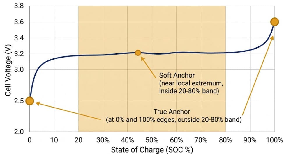
The most basic form of BMS cycle counting sets two SOC thresholds, typically near 95% and 5%. Firmware then adds one to a counter each time the pack completes a full traverse between them. This approach is cheap to build and easy to explain. As a result, it shows up often in low-cost consumer BMS platforms.
For stationary BESS, though, this method falls short. Most BESS installations rarely complete a true top-to-bottom swing. Dispatch strategies deliberately avoid the SOC extremes to protect cycle life (see our guide on the 20/80 rule for batteries). Consequently, a system cycling between 20% and 80% SOC may never trigger a single “full cycle” under this method. That can happen even after years of heavy use. This undercount is precisely why the industry moved toward throughput-based BMS cycle counting instead.
3. Method 2: BMS Cycle Counting With Ah-Throughput (EFC)
This method sits behind almost every commercial BESS warranty. Rather than watching for full swings, the BMS integrates current over time. It uses the same Coulomb-counting math built for SOC estimation. In other words, it adds up every amp-hour that flows in or out of the pack, in either direction. The BMS then divides that cumulative throughput by the pack’s rated capacity. The result is Equivalent Full Cycles, or EFC.
For example, a 500 kWh BESS that has processed 1,000 kWh of cumulative throughput has logged 2 EFC. This version of BMS cycle counting is simple. In addition, it is cheap to run continuously. And it works no matter how the pack is actually cycled, since it never requires a full 100–0% swing.
The Core Blind Spot of EFC Tracking
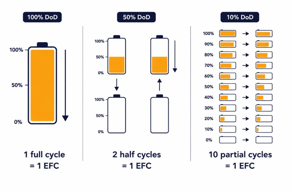
EFC has one well-known limitation: it treats every amp-hour the same, no matter how deep the swing was. As Energy-Storage.News notes, EFC alone cannot tell one cycle at 100% depth of discharge apart from two cycles at 50% DoD, or ten cycles at 10% DoD. Yet these three patterns stress the cell chemistry quite differently. So, shallow frequent cycling and deep infrequent cycling can log an identical EFC number. Even so, they age the pack at very different rates.
Many BMS platforms partly correct for this. They re-base the EFC denominator against current estimated capacity instead of nameplate capacity. That keeps the figure accurate as the pack fades. Even so, the core blind spot remains. This gap is exactly what rainflow-based BMS cycle counting was built to close.
4. Method 3: Rainflow-Based BMS Cycle Counting for Partial Cycles
Rainflow counting began as a tool for mechanical fatigue analysis. Engineers used it to turn a noisy load history into a clean set of discrete stress cycles. Battery researchers later adapted the same logic for SOC traces. A peer-reviewed ScienceDirect study on grid-integrated BESS cycle counting confirms it as the most widely used cycle-counting algorithm in the field today. Rainflow-based BMS cycle counting solves what EFC cannot: it identifies the depth of every individual swing, not just the running total.
How the Rainflow Algorithm Works Step-by-Step
The BMS records every local extremum in the SOC trace. In other words, it logs every point where the pack switches from charging to discharging, or back again.
It then calculates the SOC delta between each set of three consecutive extrema.
Consequently, If the middle delta is smaller than or equal to both neighbours, that segment counts as one closed, complete cycle at that specific depth.
The BMS removes those two points. Then it repeats the comparison on the remaining trace — much like water draining off a stepped rooftop, which is where the algorithm gets its name.
The output is a list of discrete cycles, each tagged with its own depth of discharge. For example: “47 cycles at ~80% DoD, 1,200 cycles at ~15% DoD,” instead of one flattened EFC figure.
One detail matters here: rainflow-based BMS cycle counting applies to depth of discharge, not absolute SOC. A swing from 80% down to 70% and a swing from 20% down to 10% both register as the same 10%-DoD event. Both count as equivalent stress. This lines up with how degradation models actually work, since most treat wear as a function of cycle depth, not the absolute SOC band it happens in.
Because rainflow output preserves depth data, it feeds straight into the DoD-weighted models used by SOH and RUL algorithms. That is the same layer we cover in our guide to BMS algorithms explained.
5. Method 4: Stress-Weighted BMS Cycle Counting
The most advanced BMS and EMS platforms push rainflow-based BMS cycle counting one step further. Instead of tallying cycles by depth alone, each identified cycle passes through a stress function. That function also factors in the C-rate and cell temperature present during that specific cycle. For instance, a 60%-DoD cycle at 0.2C and 25°C is far gentler than the same 60%-DoD cycle at 1.5C and 40°C. A stress-weighted counter reflects that difference clearly.
Rather than reporting a raw cycle count, this method builds a running “degradation” or “aging” score. That score, not the raw EFC number, feeds the most accurate RUL models. This is also why two BESS units with an identical EFC count can end up with very different projected remaining life.
6. How Firmware Filters Noise Before BMS Cycle Counting Begins
Raw current-sensor data is noisy. Grid-frequency jitter, brief EMS corrections, and normal sensor tolerance all create tiny, meaningless direction reversals in the SOC trace. Sometimes there are hundreds per hour. Feed that data straight into a rainflow algorithm, and the result is an explosion of trivial micro-cycles. Those micro-cycles overstate wear.
To prevent this, production BMS cycle counting firmware applies a minimum-delta, or hysteresis, threshold. A direction reversal only counts as a genuine local extremum once SOC has moved by some minimum amount, commonly 1–2%. Only then does it enter the counting algorithm. Firmware treats smaller reversals as noise and ignores them.
This single design choice separates a BMS that produces warranty-defensible cycle data from one that does not. Set the threshold too low, and cycle counts inflate from sensor noise. Set it too high, and the BMS misses genuine shallow cycling that still adds to ageing. Therefore, always ask your BMS supplier what hysteresis threshold their firmware applies. Datasheets rarely publish this figure. Yet it directly shapes every downstream SOH and warranty number.
7. Comparing the Four Cycle-Tracking Methods
Method
What It Captures
DoD-Aware?
Best For
Main Limitation
Threshold counting
Full 95%–5% traverses only
No
Simple consumer packs
Badly undercounts partial-cycling BESS
Ah-throughput (EFC)
Cumulative current throughput
No
Warranty reporting, simple dispatch
Cannot distinguish deep vs. shallow cycling
Rainflow counting
Each discrete swing, by depth
Yes
SOH modelling, mixed dispatch profiles
More compute-intensive; needs clean extrema
Stress-weighted counting
Depth + C-rate + temperature
Yes
RUL prediction, warranty defensibility
Requires a validated stress model per cell type
Most premium BMS platforms do not rely on just one method. Instead, they report EFC for simple dashboards and warranty tracking. Meanwhile, they run rainflow and stress-weighted BMS cycle counting in the background to feed SOH and RUL models. If a supplier says their BMS “counts cycles” without naming a method, ask directly. The gap between threshold counting and stress-weighted rainflow counting can differ by an order of magnitude in reported wear.
8. Why Datasheet Numbers Rarely Match Real-World Wear
A supplier’s “6,000 cycles to 80% SOH” claim is almost always a lab-derived EFC figure. Labs measure it under fixed, controlled conditions. That means a specific depth of discharge, often 80–90%, a specific C-rate, often 0.5C–1C, and a specific ambient temperature, often 25°C. Change any one of these variables in the field, and the real cycle-life outcome shifts. Sometimes it shifts substantially. We cover this relationship in detail in our guide to how temperature affects LFP battery cycle life. You can also model your own scenario with our battery cycle life calculator. For a broader reference on stationary lithium battery testing conditions, see IEC’s battery safety and performance standards.
In practice, your BMS’s in-field EFC or rainflow-weighted count measures a different operating profile than the datasheet number. A BESS running frequent shallow cycles at moderate temperature may outlive its rated cycle count in calendar terms. Meanwhile, one running deep cycles at high ambient temperature may fall short of it. Neither outcome means the datasheet number was wrong. It simply means BMS cycle counting and lab-rated cycle life measure two related, but distinct, things.
9. Questions to Ask About Your Supplier’s BMS Cycle Counting Method
Which cycle-counting method does the firmware run: threshold, raw EFC, rainflow, or stress-weighted? A BMS that only reports raw EFC cannot show how deep-cycling patterns affect real degradation.
What minimum-delta, or hysteresis, threshold filters noise before a reversal counts as a cycle? An unpublished or unreasonably low threshold can quietly inflate cycle counts.
Is the EFC denominator based on nameplate capacity or current estimated capacity? Using nameplate capacity for the pack’s whole life understates EFC as the cell ages.
Does the cycle-counting output feed the SOH and RUL algorithms directly, or are they calculated separately? Disconnected pipelines often cause inconsistent SOH and warranty reporting.
What DoD, C-rate, and temperature conditions does the warranty’s rated cycle-life figure assume? This baseline is what your field cycle count should be compared against, not treated as a universal number.
Consider a 100 kWh BESS module running a frequency-regulation profile for one day. It discharges 8 kWh, charges 5 kWh, discharges 12 kWh, charges 10 kWh, discharges 6 kWh, and charges 9 kWh. That adds up to 50 kWh of cumulative throughput.
Decomposed into 3 discrete cycles at ~8%, ~12%, ~9% DoD
3 shallow cycles logged, none flattened into one number
While both numbers are technically correct, they answer different questions. The 0.50 EFC figure shows up on a simple throughput dashboard and feeds warranty-cycle tracking. The rainflow breakdown, however, is what a SOH model actually needs. Three shallow 8–12% DoD cycles age a cell differently than one 50%-DoD cycle would. That holds true even though both scenarios can produce the same EFC total.
Conclusion: BMS Cycle Counting Is a Modelling Choice, Not a Simple Tally
A BMS does not count cycles the way a person counts laps around a track. Instead, it reconstructs a cycle metric from a continuous current and SOC trace. Each method trades simplicity for accuracy differently. Threshold counting is too crude for real BESS dispatch. EFC is the industry-standard warranty metric, yet it stays blind to depth of discharge. Rainflow-based BMS cycle counting recovers that missing depth information. It breaks messy, real-world SOC traces into discrete, weighted cycles. Stress-weighted counting goes further still. It folds in C-rate and temperature to build the aging score that actually drives accurate RUL prediction.
For BESS buyers and operators, the lesson is simple. Do not take “the BMS tracks cycle count” at face value. Instead, ask which method it uses. Ask how it filters sensor noise. And ask how that number connects to the SOH and RUL figures you will eventually rely on for warranty claims and second-life valuation.
☀️ Need a BMS Cycle Counting and SOH Methodology Review? SunLith Energy reviews BMS cycle counting implementation, EFC and rainflow methodology, and SOH-RUL linkage for BESS projects from 50 kWh upward. Contact us before you commit to a supplier.
Frequently Asked Questions
How does BMS cycle counting work?
BMS cycle counting converts raw current and SOC data into a wear metric. Most systems first calculate cumulative Ah or kWh throughput. They then convert it into Equivalent Full Cycles. More advanced platforms add a rainflow algorithm on top. It breaks the SOC trace into discrete cycles at their true depth of discharge, filtering out small reversals below a set noise threshold.
What is an Equivalent Full Cycle (EFC) in BMS cycle counting?
An EFC is the standard unit behind most BMS cycle counting for warranty purposes. The BMS sums all Ah or kWh throughput — every unit of charge or discharge, in either direction. It then divides that total by the pack’s rated or current estimated capacity. Two cycles at 50% depth of discharge, and one cycle at 100% depth of discharge, both produce 1 EFC.
Why does depth of discharge matter if EFC already tracks total throughput?
Because EFC only tracks the total charge moved, not how it was distributed. A cell that goes through one deep 100%-DoD cycle experiences different stress than one that goes through ten shallow 10%-DoD cycles. Yet both can produce the same EFC total. Rainflow-based BMS cycle counting exists specifically to preserve this depth information for accurate SOH and RUL modelling.
What is rainflow counting, and why does BMS cycle counting use it?
Rainflow counting is an algorithm first built for mechanical fatigue analysis. Applied to a battery’s SOC trace, it identifies local turning points. It then pairs them into discrete, complete cycles at their true depth of discharge, instead of one flattened throughput number. This makes it the preferred method for BMS cycle counting on BESS platforms with irregular, partial-cycling dispatch profiles.
Why doesn’t my BESS ever seem to reach the cycle count on its datasheet?
The datasheet figure is almost always measured under fixed lab conditions: a specific depth of discharge, C-rate, and temperature. If your system cycles more shallowly, at a gentler C-rate, or at cooler temperatures, its real-world BMS cycle counting output accumulates more slowly than the lab figure implies. The reverse is true under harsher conditions.
Can two BESS units show the same cycle count but have different remaining life?
Yes. Raw EFC, and even simple cycle counts, do not capture the temperature and C-rate conditions each cycle occurred under. This is why advanced BMS cycle counting adds a stress-weighted layer. It produces a degradation score rather than a plain cycle number, which feeds more accurate Remaining Useful Life predictions than cycle count alone.
⚡ Quick Answer: What Are BMS Algorithms? BMS algorithms go far beyond SOC estimation. A production BMS runs several algorithms at once: SOH estimation, SoP, SoE, cell balancing logic, contactor sequencing, isolation monitoring, safety diagnostics, and RUL prediction. For BESS, the quality of these BMS algorithms decides dispatch reliability, warranty defensibility, and second-life value — not just SOC accuracy.
1. Beyond SOC: The Full BMS Algorithm Stack
Most talk about BMS algorithms stops at State of Charge. SOC matters. But it is only one output from a stack of six or more BMS algorithms running at once.
For a deeper dive into OCV lookup, Coulomb counting, and Extended Kalman Filter SOC methods, see our dedicated guide: BMS SOC Estimation Methods Explained. This article picks up where those leave off, covering the advanced firmware algorithms that drive aging, dispatch limits, safety, and long-term asset value.
A BESS operator or EPC should understand what each BMS algorithm actually calculates. Marketing language often overstates what firmware really runs. The sections below walk through each algorithm layer in build order: health first, then power and energy limits, then balancing, then safety, then long-term prediction.
2. SOH Algorithms: How BMS Algorithms Track Battery Aging
State of Health (SOH) is the second most important number a BMS produces after SOC. It is also far harder to calculate correctly. SOH shows how much usable capacity and performance remain compared to a new cell. A cell rated at 100 Ah that now delivers 92 Ah has an SOH of roughly 92%.
Unlike SOC, SOH cannot reset with one charge cycle. The BMS must infer it from long-term trends. This makes SOH-focused BMS algorithms fundamentally different from SOC algorithms.
Capacity Fade Tracking Algorithm
The simplest SOH algorithm compares measured full-charge capacity against rated nameplate capacity. The BMS records the Ah delivered between two known SOC points, typically 100% to 0%. It then compares that figure against the original rated capacity.
This method is accurate but slow. It produces one new SOH data point per full cycle. Many BESS installations rarely complete a true 100–0% cycle. Partial-cycle capacity fade algorithms estimate the fade rate from partial cycles instead, using coulomb-counted throughput and known depth-of-discharge. These partial-cycle BMS algorithms carry more uncertainty than full-cycle measurements.
Incremental Capacity Analysis (ICA) Algorithm
Incremental capacity analysis is a more advanced SOH algorithm. It examines the shape of the voltage curve, not just its endpoints. As a cell ages, specific peaks in its incremental capacity curve (dQ/dV) shift and shrink. Each shift pattern correlates with a specific degradation mechanism: lithium plating, active material loss, or electrolyte decomposition.
ICA-based BMS algorithms can tell different aging causes apart, not just report one percentage. This matters for warranty claims and second-life valuation. A cell degrading from normal calendar aging is a very different asset than one degrading from a manufacturing defect or thermal abuse event.
The tradeoff is cost. ICA needs high-resolution voltage sampling during specific charge segments. Not every BMS platform captures this data by default.
DCIR-Based SOH Algorithm
DC internal resistance (DCIR) rises as a cell ages, mostly independent of capacity fade. A DCIR-based SOH algorithm applies a known current pulse and measures the resulting voltage drop. It then calculates internal resistance using Ohm’s law, and compares that value against a baseline resistance-versus-age curve for the specific cell model.
DCIR-based SOH algorithms run faster than capacity-fade methods, since a short current pulse is enough — no full cycle required. This makes them useful for spotting outlier cells early, often before capacity fade becomes visible.
The limitation is temperature sensitivity. DCIR shifts a lot with cell temperature. An accurate DCIR-based BMS algorithm must correct every reading against a resistance-versus-temperature-versus-age model calibrated for the exact cell in use.
SOH Algorithm Comparison
Method
What It Measures
Update Frequency
Best For
Capacity fade tracking
Ah delivered vs. rated capacity
Once per full cycle
Systems with regular full cycles
Incremental capacity analysis (ICA)
dQ/dV curve shape and peak shift
Per qualifying charge segment
Distinguishing aging mechanisms, warranty claims
DCIR-based SOH
Internal resistance rise vs. baseline
Per current pulse (fast)
Early outlier-cell detection, partial-cycle systems
Most premium BMS platforms combine all three algorithms: DCIR for fast, frequent checks; capacity fade tracking as the long-term anchor; and ICA for diagnostic deep-dives when a cell shows early warning signs.
3. SoP Algorithm: What BMS Algorithms Tell the Inverter
State of Power answers a different question than SOC or SOH. It asks not “how much energy is stored,” but “how much power can this pack safely deliver or accept right now.” The SoP algorithm calculates the maximum charge and discharge power available for a set time window, typically 1, 10, or 30 seconds. It weighs current SOC, temperature, cell voltage limits, and internal resistance.
This number goes straight to the inverter or PCS and to the energy management system (EMS). Without an accurate SoP algorithm, the EMS either under-dispatches or over-dispatches. Under-dispatching leaves revenue on the table during a frequency regulation or peak-shaving event. Over-dispatching triggers a protection cutoff mid-event, which is worse for grid-service contract compliance.
SoP gets harder to calculate at temperature and SOC extremes. A pack at 10% SOC or −5°C has much lower discharge SoP than the same pack at 50% SOC and 25°C, even with similar energy content. A well-designed SoP algorithm accounts for voltage sag under load. It does not rely on static cell voltage limits alone, and it uses the same internal resistance data the SOH algorithm tracks.
4. SoE Algorithm: Usable kWh, Not Just Percentage
SOC gives you a percentage. The SoE algorithm gives you the actual usable kilowatt-hours remaining. It factors in current SOH, temperature derating, and the depth-of-discharge limits set for the system. Two BESS units showing 60% SOC can have very different SoE if one has degraded to 85% SOH and the other sits near 98% SOH.
For asset owners running dispatch contracts or virtual power plant participation, SoE is the number that actually sets revenue capacity. A BMS that only reports SOC forces the EMS to apply a separate correction factor for aging, and that workaround adds error. A BMS with a proper SoE algorithm reports usable energy directly, already corrected for real-world capacity.
5. SoR and SoF Algorithms: Diagnostic and Dispatch-Readiness Checks
Two less-discussed BMS algorithms round out the state-estimation stack.
State of Resistance (SoR) tracks internal resistance as its own diagnostic metric, separate from its role as a SOH input. Rising resistance in a single string or module is often the earliest sign of an emerging fault. It can flag a loose busbar connection or accelerated local aging before it shows up in the pack-level SOH number.
State of Function (SoF) is a composite go/no-go algorithm. It combines SOC, SOH, SoP, temperature, and active fault flags into one dispatch-readiness signal. The EMS checks this signal before committing the BESS to a grid-service event. A pack can have fine SOC and SOH individually and still fail SoF — for example, if a temperature sensor reads near its fault threshold. SoF exists to stop the EMS from dispatching a unit that has energy on paper but should not be trusted for that event.
6. Cell Balancing Algorithms: Passive vs Active Control Logic
Cell balancing keeps every cell in a series string at a matched voltage and SOC. The control logic behind it is itself a BMS algorithm worth understanding, not just a hardware feature.
This balancing logic is especially vital—and complex—when dealing with the flat voltage plateaus of LFP chemistry; for a deeper look at hardware and balancing nuances there, read our specific guide on BMS for LiFePO4 batteries.
Passive Balancing Algorithm Logic
A passive balancing algorithm finds the highest-voltage cell in a string during charge. It then switches a bleed resistor across that cell, burning off excess energy as heat until the cell matches the pack average. The control logic usually triggers balancing only above a voltage or SOC threshold, commonly near the top of charge, where cell mismatch matters most for safety and full-charge capacity.
Design choices matter more than the hardware here. A poorly tuned threshold balances too aggressively, wasting energy and building unnecessary heat. Too conservative a threshold lets mismatch build up for many cycles.
Active Balancing Algorithm Logic
An active balancing algorithm moves charge from higher-voltage cells to lower-voltage cells, using inductors, capacitors, or switched-capacitor networks. It does not just burn off the difference as heat. The control logic is more complex: it must sequence several transfer paths at once, avoid oscillation between cells close in voltage, and decide when further balancing no longer justifies the switching losses.
For grid-scale BESS with thousands of series-parallel cells, the balancing algorithm’s efficiency affects round-trip efficiency and effective cycle life directly. A well-balanced pack ages its weakest cells more slowly, since those cells spend less time at voltage extremes.
7. Contactor and Isolation BMS Algorithms
Two safety-critical BMS algorithms operate below the level most BMS content ever discusses. They matter a great deal for BESS commissioning and daily operation.
Pre-Charge Sequencing Algorithm
When a BESS connects to its inverter or DC bus, a large voltage gap between the battery and a discharged bus can spike current high enough to weld contactor contacts or blow fuses. The pre-charge sequencing algorithm closes a smaller pre-charge contactor through a current-limiting resistor first. It watches the bus voltage rise toward battery voltage, and only closes the main contactor once the gap falls within a safe threshold, typically a few percent.
The algorithm must also set a timeout and a fault response. If bus voltage fails to rise as expected in time, that signals a downstream fault. A well-designed sequence aborts the connection instead of forcing the main contactor closed anyway.
Isolation Monitoring Algorithm
High-voltage BESS strings must stay electrically isolated from chassis ground. The isolation monitoring algorithm injects a small test signal, or measures leakage current, between the HV bus and chassis ground. It then calculates an isolation resistance value. A common safety threshold is 500 ohms per volt of system voltage — a 750V BESS string needs at least 375,000 ohms of isolation resistance under this rule.
A slowly degrading isolation reading, even one still above the fault threshold, is an early warning worth flagging. It usually points to moisture ingress, insulation wear, or a developing ground fault well before it trips a hard fault.
8. Safety Diagnostic Algorithms: MAVD, RdV, and Early Fault Detection
Beyond voltage, current, and temperature thresholds, advanced BMS platforms run pattern-based diagnostic algorithms. These catch failure modes before they reach a hard safety limit.
Maximum Allowable Voltage Deviation (MAVD) algorithms compare each cell’s voltage against the pack average in real time. A cell drifting outside its expected deviation band can signal an internal short, a connection fault, or local degradation — even while it stays within absolute safe voltage limits. Because MAVD looks at relative deviation, not absolute thresholds, it often catches faults earlier than simple over-voltage or under-voltage protection.
Resistance-derivative or rate-of-change (RdV) algorithms track how fast a cell’s voltage or resistance is changing, not just its current value. A cell with rapidly climbing resistance is a different risk than one with stable but elevated resistance, even if both report the same SOH today. RdV algorithms flag the rate of change itself as its own alarm condition.
These diagnostic layers matter most for large-format BESS, where a single degrading cell among thousands can go unnoticed until it causes a string-level fault. Standards bodies such as the IEC publish safety requirements for stationary lithium battery systems that reference exactly this kind of deviation monitoring.
Furthermore, if you are deploying assets in the European market, these algorithmic diagnostics are critical for compliance; see our EU batteries regulation EU 2023 1542 complete guide for a full breakdown of the data and safety mandates.
Ask suppliers whether their BMS runs deviation and rate-of-change diagnostics on top of standard threshold protections — this is a real differentiator between a basic BMS and a genuinely safety-engineered one.
9. RUL Prediction Algorithms and Second-Life Value
Remaining Useful Life algorithms take SOH trend data and project forward. They estimate how many more cycles or years remain before the pack falls below an end-of-life threshold, commonly 70–80% of original capacity.
Three RUL Algorithm Approaches
Empirical RUL algorithms fit a degradation curve — often exponential, or a two-stage linear-then-accelerating shape — to historical SOH data for the specific chemistry and use profile. They then extrapolate forward. These are cheap to run and reasonably accurate for well-studied LiFePO4 chemistries with large datasets for a quick way to model these degradation curves yourself based on cycle depth and temperature, you can check out our interactive battery cycle life calculator. But they assume future use resembles the past.
Physics-based (electrochemical) RUL algorithms simulate the degradation mechanisms directly: lithium plating, SEI growth, active material loss. They predict RUL from first principles. These are more accurate under changing use conditions, but they need detailed cell-level parameters that cell suppliers do not always share.
Machine-learning RUL algorithms train on large fleets of historical degradation data. They predict RUL from current sensor patterns without an explicit physical or empirical formula. These can beat both other approaches when trained on a large enough fleet of the same cell type and use case. But they need a lot of historical data, and they can behave unpredictably outside the conditions they trained on.
Why RUL Algorithm Accuracy Matters for BESS Economics
RUL accuracy affects two commercial decisions directly: warranty reserve calculations for suppliers, and second-life asset valuation for owners. A BESS pack projected to hold 80% capacity for ten more years is worth much more on the second-life market than one with an uncertain or steeply declining RUL curve. Lower-demand second-life uses, like residential backup or slow-cycling grid support, depend on that projection being credible.
For utility-scale BESS operators planning eventual asset disposition, ask your BMS or EMS supplier which RUL modeling approach they use, and what fleet data backs it. Battery aging research from national labs such as NLR (National Laboratory of the Rockies) increasingly informs these models. Ask whether RUL confidence intervals are reported alongside the point estimate — a single RUL number with no range is hard to use for financial planning.
10. Questions to Ask Your BMS Supplier About Algorithms
Marketing language often claims “advanced algorithms” without saying which ones actually run in firmware. For a structured framework on auditing these capabilities during procurement, see our guide on BESS supplier BMS evaluation.
The following targeted questions will help you separate real algorithmic depth from a basic protection-only BMS with technical-sounding labels:
Which SOH algorithm does the BMS use — capacity fade tracking, ICA, DCIR-based, or a combination? A BMS that only runs capacity fade tracking will be slow to catch outlier cells in systems that rarely complete full cycles.
Does the BMS calculate SoP and SoE algorithms, or only SOC and SOH? Without SoP output, the EMS must apply conservative blanket power limits, which lowers dispatch revenue.
What isolation resistance threshold does the algorithm enforce, and how is it temperature- and time-compensated? A static threshold with no trend monitoring misses slow isolation decay.
Does the balancing algorithm run passive, active, or both, and what triggers a balancing cycle? Ask for the specific voltage or SOC threshold, not just “the BMS balances cells.”
What RUL algorithm approach is used, and is a confidence interval reported? A point-estimate RUL number with no uncertainty bounds has limited use for financial and warranty planning.
Conclusion: Algorithm Depth Is the Real BMS Differentiator
SOC estimation gets most of the attention in BMS marketing. But the BMS algorithms that actually protect a BESS investment over its 10–20 year life sit one layer deeper. SOH tracking catches aging mechanisms early. SoP and SoE outputs maximize safe dispatch revenue. Balancing logic gets tuned for the specific pack architecture. Safety diagnostics catch deviation before it becomes a fault. RUL models come with defensible confidence intervals.
When you evaluate a BMS or a BESS supplier, ask specifically which of these BMS algorithms are implemented, and how they were validated. Do not settle for “the BMS monitors SOC and SOH.” The answer reveals whether you are buying genuine algorithmic engineering or a basic protection circuit with confident marketing copy.
☀️ Need a BMS Algorithm Review for Your BESS Project? Sunlith Energy reviews BMS algorithm implementations — SOH methodology, SoP/SoE accuracy, balancing logic, and RUL modeling — for BESS projects from 50 kWh upward. Contact us before you commit to a supplier.
Frequently Asked Questions About BMS Algorithms
What algorithms does a BMS run besides SOC estimation?
A production BMS runs several algorithms beyond SOC: SOH estimation (capacity fade tracking, incremental capacity analysis, or DCIR-based methods), SoP and SoE calculations, cell balancing control logic, contactor pre-charge sequencing, isolation monitoring, safety diagnostics such as voltage-deviation and resistance-rate-of-change monitoring, and often RUL prediction models.
What is the difference between the SOH and SoP algorithms in a BMS?
The SOH algorithm measures how much capacity and performance a battery has lost compared to new, shown as a percentage. The SoP algorithm measures how much power the battery can safely deliver or accept right now, based on current SOC, temperature, and internal resistance. SOH looks backward at cumulative aging. SoP looks at the immediate power ceiling for dispatch decisions.
Why does the SoP algorithm matter for BESS dispatch even if SOC looks fine?
A pack can show good SOC while still having a low SoP at cold temperatures or high internal resistance. That means it cannot deliver the power a grid-service event needs without tripping a voltage protection limit. An EMS that only checks SOC before dispatch risks committing to an event the pack cannot actually support.
How does the DCIR-based SOH algorithm work?
The BMS applies a known current pulse and measures the resulting voltage drop. It calculates internal resistance using Ohm’s law, then compares that resistance against a temperature-compensated baseline curve for the specific cell model. This algorithm runs faster than capacity-fade tracking, since it needs no full charge-discharge cycle.
What is a good RUL algorithm confidence level for a utility-scale BESS?
There is no single universal number — it depends on the modeling approach and available fleet data. What matters more is whether the supplier reports a confidence interval at all, rather than a single point estimate, and whether the model has been checked against real fleet degradation data for the same cell chemistry and use profile.
Do I need an active balancing algorithm for a grid-scale BESS, or is passive enough?
Passive balancing works fine for many commercial and lower-cycling systems. For utility-scale BESS with high cycling frequency and large series strings, an active balancing algorithm usually improves round-trip efficiency and cuts accelerated aging in weaker cells. That can justify its added cost over the system’s lifetime.
AC-coupled vs DC-coupled BESS is one of the first choices you’ll face in any solar-plus-storage project. This one decision shapes your system’s efficiency, cost, and how easily you can expand it later. Both architectures store solar energy in a battery for later use. But they connect the battery in different places relative to the inverter, and that single design choice ripples through nearly every other spec on the system. This guide walks through the differences so you can pick the right fit.
What Is AC-Coupled BESS?
An AC-coupled BESS connects the battery to the grid through its own dedicated inverter. This component sits separate from the solar PV inverter. Power from PV and power from the battery meet on the AC side of the system rather than sharing a DC bus. This makes AC-coupled storage the more common choice when you’re adding a battery to solar you already have running. For the full breakdown of components and operation, see What is AC Coupled BESS?.
What Is DC-Coupled BESS?
A DC-coupled BESS connects the battery and the solar PV array on the same DC bus, ahead of a single shared inverter. Because both share one conversion path, DC-coupled systems typically post better round-trip efficiency and lower equipment costs, at the expense of retrofit flexibility. For the full architecture and step-by-step operation, see What is DC Coupled BESS?.
AC-Coupled vs DC-Coupled BESS: Side-by-Side Comparison
Here’s the AC-coupled vs. DC-coupled BESS comparison at a glance — the factors that matter most when you design a solar-plus-storage system:
Factor
AC-Coupled BESS
DC-Coupled BESS
Connection point
Battery connects via its own inverter on the AC side
Battery and PV share one DC bus, ahead of a single inverter
Inverters required
Two — one for PV, one for battery
One shared hybrid inverter
Conversion stages
Multiple DC-AC-DC conversions on some charge paths
Single DC-to-AC conversion for grid/load power
Round-trip efficiency
Lower — extra conversion stages add losses
Higher — fewer conversion losses
Balance-of-system cost
Lower than standalone, but higher than DC-coupled (separate inverters, switchgear)
Lowest of the three — shared inverter and BOS hardware
Best for
Retrofitting storage onto existing solar
New-build, greenfield solar-plus-storage projects
Solar charging during outage
Depends on inverter design; may need extra hardware
Typically yes, in most configurations
Curtailment / clipping capture
Limited — PV inverter still governs PV output
Can capture otherwise-clipped PV energy behind a higher-ILR array
Grid response speed
Slower — control system coordinates multiple inverters
Faster — single inverter, more direct control path
Future expansion
Easier — PV and storage can be sized/upgraded independently
Harder — added battery capacity must match existing DC bus voltage
No single architecture wins on every factor. The right choice depends on your project type and how much you weigh upfront cost against long-term efficiency.
AC-Coupled vs DC-Coupled BESS: Efficiency Compared
Every DC-to-AC conversion wastes some energy as heat. An AC-coupled system can convert PV energy to AC, then back to DC to charge the battery, then to AC again when you use it. That’s up to three conversion stages on some charge paths.
A DC-coupled system skips most of that. It charges the battery straight from the DC bus and converts to AC only once, when you actually need AC power. This is the core reason DC-coupled architectures tend to post higher round-trip efficiency in side-by-side testing.
Both architectures cost less than siting solar and storage separately. DC-coupled systems generally cost less than AC-coupled ones on new-build projects, too.
The U.S. Department of Energy’s Solar-Plus-Storage 101 resource confirms this pattern: co-locating PV and storage on the same site cuts system cost compared to siting them separately, whether you choose AC-coupled or DC-coupled. Most of the savings come from shared balance-of-plant infrastructure.
DC-coupled designs push those savings further. They eliminate a full second inverter and its switchgear. That said, retrofit constraints can narrow this advantage — if AC-coupling is your only practical option, the smaller cost gap may not matter much.
Retrofit vs. Greenfield: Matching Architecture to Project Stage
Project stage often decides the outcome before cost or efficiency even enter the conversation.
If you already run solar, adding a DC-coupled battery means tying into the existing DC bus and matching its voltage. That’s technically possible, but it usually means replacing or reconfiguring your existing inverter. AC-coupled storage sidesteps that problem entirely — the battery gets its own inverter and connects on the AC side, so your existing solar installation stays untouched.
New-build, greenfield projects don’t face that constraint, since you design PV and storage together from day one. That’s why DC-coupled architectures dominate new utility-scale and C&I builds. In the end, this AC-coupled vs. DC-coupled BESS decision usually comes down to one question: are you retrofitting, or building new?
When to Choose AC-Coupled BESS
Adding storage to solar you already have running
Projects where you need to size, optimize, or replace PV and battery independently
Sites where minimizing changes to existing PV wiring and permits matters
Phased projects that add storage well after the solar installation
Systems needing simpler expansion of storage capacity over time
When to Choose DC-Coupled BESS
New solar-plus-storage builds where you design PV and storage together from the start
Utility-scale and C&I projects prioritizing round-trip efficiency
Microgrid and off-grid systems needing solar charging during outages
High inverter-loading-ratio PV arrays looking to capture otherwise-clipped energy
Projects where minimizing equipment count and balance-of-system cost is a priority
AC-Coupled vs DC-Coupled BESS: Trade-offs to Weigh
Efficiency and cost aren’t the only variables to weigh.
DC-coupled systems can be harder to expand later. Additional battery capacity generally needs to match the voltage of your existing DC bus. The tighter integration between PV and storage also means a fault on one side can affect the other.
AC-coupled systems avoid that coupling risk and expand more easily. You pay for that flexibility with two inverters, two sets of switchgear, and a somewhat slower response to fast grid commands like frequency regulation, since the control system has to coordinate multiple inverters instead of one.
Weigh these trade-offs against your project’s timeline, budget, and growth plans. That usually beats picking the ‘better’ architecture in the abstract.
Can You Combine AC-Coupled and DC-Coupled BESS?
Some projects don’t have to choose only one. A hybrid architecture can pair DC-coupled storage on a new PV block with an existing AC-coupled asset elsewhere on-site. Or it can phase in DC-coupled storage over multiple project stages. You’ll see this more often on larger utility-scale sites with modular BESS designs. For a broader look at how AC-coupled, DC-coupled, modular, and hybrid designs fit together, see our guide to Understanding Energy Storage System BESS Architectures.
Frequently Asked Questions
Here are quick answers to the AC-coupled vs DC-coupled BESS questions we hear most often:
What is the main difference between AC-coupled and DC-coupled BESS?
AC-coupled systems use two separate inverters — one for solar PV and one for the battery. DC-coupled systems share a single inverter. PV and battery connect to the same DC bus before the system converts power to AC.
Which is more efficient, AC-coupled or DC-coupled BESS?
DC-coupled BESS is generally more efficient because energy converts from DC to AC only once. AC-coupled systems often involve extra conversion stages, especially when charging the battery from solar, and that raises round-trip losses.
Is AC-coupled or DC-coupled BESS cheaper?
DC-coupled systems typically cost less on the balance-of-system side, since they need only one inverter and one set of switchgear. AC-coupled systems cost more upfront, but you can add them incrementally, which sometimes offsets the gap on retrofit projects.
Can I add a DC-coupled battery to an existing solar system?
You can, but it’s more complex than AC-coupling. The battery must connect to the existing DC bus and match its voltage. For most retrofits, AC-coupled storage is the simpler, more common approach.
Does DC-coupled BESS work off-grid?
Yes. DC-coupled architectures generally support off-grid and islanded operation. They can keep charging from solar during a grid outage, which makes them a common choice for microgrid and remote projects.
Why do DC-coupled systems capture more solar energy?
In a DC-coupled system, the battery can charge directly from PV output that would otherwise get clipped when the inverter loading ratio exceeds 1. That’s because the battery sits on the DC side, before the inverter’s AC output limit applies.
Is there a hybrid option that combines AC and DC coupling?
Yes. Some larger projects use a hybrid architecture that pairs DC-coupled storage with an existing AC-coupled asset, or phases DC-coupled storage in over time. You’ll see this more often on utility-scale sites with modular BESS designs.
AC-Coupled vs DC-Coupled BESS: Final Verdict
AC-coupled and DC-coupled BESS both store solar energy for later use, but they get there differently. That difference shows up in efficiency, cost, and how easily the system grows over time.
AC-coupled storage stays the more flexible choice for retrofits and phased projects. DC-coupled architectures tend to win on efficiency and cost for new-build solar-plus-storage systems. The right call comes down to where your project starts, not which architecture is objectively ‘better’.
Whichever direction fits your project, the Sunlith Energy team can help size and specify the right BESS architecture, PCS, and battery configuration for your site.
Power outages cost businesses billions every year. Aging grid infrastructure, extreme weather, and the variable nature of solar and wind energy make centralized power systems less reliable. As a result, energy-forward organizations are turning to microgrid BESS — a combination of distributed energy resources and battery storage that can supply power independently of the utility grid.
A microgrid BESS is not simply a backup generator. Instead, it is an intelligent energy platform that stores renewable energy, dispatches it on demand, and switches smoothly between grid-connected and islanded operation. To understand the foundation of this technology, read our ultimate guide to battery energy storage systems before diving into the microgrid-specific details covered here.
This guide covers everything EPCs, project developers, and commercial energy buyers need to know. Topics include: how these systems work, core components, sizing methodology, use cases, grid-forming technology, relevant standards, and financial considerations.
What Is a Microgrid BESS?
A microgrid is a local energy network. It integrates distributed energy resources — solar PV, wind turbines, diesel generators, and battery storage — into one controllable system. Crucially, it can run in two modes: grid-connected (exchanging power with the utility) or islanded (supplying loads on its own).
Battery storage is the technology that makes islanded operation practical. Without BESS, a microgrid relying on solar cannot guarantee stable voltage and frequency when it disconnects from the grid. With BESS, however, the system buffers generation gaps, sustains loads overnight, and holds the frequency reference that other devices need. For a broader look at how BESS works across sectors, see our guide on top applications of commercial and industrial BESS.
In short: BESS is the backbone of a modern microgrid. It turns a set of distributed generators into a self-sufficient power system.
Grid-Connected vs. Islanded Microgrid BESS
Microgrid BESS Operating Modes — Grid-Connected vs. Islanded
Microgrid BESS operates in two fundamental modes. Understanding both is essential before sizing or specifying a system.
Grid-connected mode: The microgrid stays synchronized with the utility. BESS handles peak shaving, load shifting, and frequency regulation. Excess solar generation is stored or exported.
Islanded (off-grid) mode: The microgrid disconnects at the point of common coupling. BESS then acts as the voltage reference, sustaining all local loads entirely on its own.
Seamless transition between these modes is a critical performance target. Research published in Energies (2026) showed loss-of-mains detection in under 3 milliseconds — well within the 10-millisecond threshold needed for sensitive equipment to ride through without disruption.
Core Components of a Microgrid BESS System
A complete microgrid BESS integrates several interdependent subsystems. Knowing each one helps EPCs design reliable systems and helps project developers evaluate vendor proposals accurately.
1. Battery Modules and Racks — LFP Chemistry
Lithium Iron Phosphate (LFP) chemistry dominates microgrid deployments today. LFP delivers over 6,000 cycles at 80% depth of discharge. It also operates safely across wide temperature ranges and avoids the thermal runaway risk seen in NMC chemistry. Battery modules are assembled into racks and housed in containerized enclosures for rapid site deployment.
2. Battery Management System (BMS)
The BMS monitors cell-level voltage, temperature, and current. It enforces SoC limits (typically 20–80% under the 20/80 cycling rule), calculates State of Health (SoH), and tracks DC Internal Resistance (DCIR). Additionally, the BMS communicates with the EMS via CAN bus or Modbus. For a deeper look at how the EMS works inside a BESS, we have a dedicated technical article on the subject.
3. Power Conversion System (PCS)
The PCS — also called the bidirectional inverter — converts DC energy from batteries into AC power for loads. It also converts AC to DC during charging. In a microgrid, the PCS can operate in grid-following or grid-forming mode. Grid-forming units synthesize voltage and frequency from scratch, which makes islanded operation possible even without a utility reference.
4. Energy Management System (EMS)
The EMS is the intelligence layer. It receives data from the BMS, PCS, solar inverters, load meters, and weather forecasts. Then it dispatches charge/discharge commands to optimize across multiple objectives simultaneously — peak shaving, renewable self-consumption, SoC management, and grid services. Moreover, it governs mode transitions and coordinates load shedding during generation shortfalls. Read our full breakdown of how EMS enables advanced grid services through BESS to see exactly how this works in practice.
5. Solar PV Array
Solar PV is the primary generation source in most microgrid BESS deployments. The PV array charges the BESS during daylight hours. As a result, the BESS can supply loads through the night or during cloud cover. Oversizing the PV-to-BESS ratio — typically 1.2× to 1.5× — ensures adequate charging under real-world irradiance conditions.
6. Point of Common Coupling (PCC) Switch / STS
The PCC switch or Static Transfer Switch (STS) is the electrical boundary between the microgrid and the utility grid. During a grid disturbance, the STS opens within milliseconds to island the microgrid. When grid power returns and stabilizes, the STS synchronizes and re-closes. Consequently, the speed and reliability of this device directly determines the quality of power continuity during transitions.
Microgrid BESS Component Summary Table
Component
Primary Function
Key Standard
Typical Technology
Battery Module
Store DC energy
IEC 62619, UL 1973
LFP, NMC
BMS
Cell monitoring, protection, SoH tracking
IEC 62133-2
Rack-level + pack-level
PCS / Inverter
DC↔AC conversion, grid forming/following
IEEE 1547, UL 1741
Grid-forming (VSM/droop)
EMS
Dispatch, optimization, mode transitions
IEC 62933-5-2
SCADA + AI forecasting
STS / PCC Switch
Grid isolation, mode transition
IEEE 1547.4
<20 ms transfer
Solar PV Array
Primary renewable generation
IEC 61215, IEC 61730
Monocrystalline TOPCon
Thermal Management
Temperature control, fire suppression
NFPA 855, UL 9540A
HVAC + liquid cooling
Microgrid BESS Components Architecture Diagram
Grid-Forming BESS: The Key to True Islanding
The most important technology choice in any microgrid BESS project is the inverter control mode. Specifically, you must decide between grid-following and grid-forming. This single decision determines whether the system can operate independently of the utility at all. Our detailed grid-forming vs. grid-following BESS guide covers the full technical comparison, but the key points are summarized below.
Grid-Following BESS: Its Core Limitation
A grid-following inverter acts as a current source. It detects the voltage and frequency of an active grid and synchronizes its output to that reference. Therefore, if the grid disappears — during a blackout — a grid-following inverter cannot sustain islanded operation. It must shut down immediately per IEEE 1547 anti-islanding requirements to protect utility workers.
This means a grid-following BESS cannot black-start a dead network. Nor can it sustain an islanded microgrid on its own. As a result, it is not a viable standalone solution for resilience-critical sites.
Grid-Forming BESS: How It Creates the Grid
Grid-Forming vs Grid-Following BESS Inverter Comparison
A grid-forming inverter operates as a voltage source instead. Rather than following an external signal, it synthesizes its own voltage waveform and frequency using algorithms such as Virtual Synchronous Machine (VSM) or droop control. Consequently, all devices on the microgrid — other inverters, loads, generators — synchronize to the grid-forming BESS.
This fundamental shift in control architecture unlocks four critical capabilities:
Black start: The grid-forming BESS energizes a completely dead network from zero.
Sustained islanding: The microgrid runs indefinitely without any utility connection.
Synthetic inertia: The inverter emulates the rotational inertia of a synchronous generator, stabilizing frequency during rapid load changes.
Fault current contribution: The system provides enough fault current to trip protection relays, enabling conventional protection coordination.
As of mid-2025, Australia had deployed 1,070 MW of grid-forming BESS across ten sites, according to AEMO. Furthermore, a 2025 Nature Scientific Reports study confirmed that integrated grid-forming inverter strategies significantly improve microgrid resilience under fault conditions. This real-world track record proves that grid-forming technology is no longer experimental.
How to Size a Microgrid BESSSystem
Getting the size right is critical. An undersized system fails to cover loads overnight or during weather events. An oversized system wastes capital. Fortunately, the sizing methodology follows four clear, sequential steps.
Step 1 — Establish the Load Profile
Start with a complete energy audit. Measure peak demand (kW) and daily energy consumption (kWh). Identify critical loads that must run during islanding and non-critical loads that can be shed. Also account for motor start-up inrush currents, which can reach 6× running current and must be covered by the PCS peak power rating.
Step 2 — Define Autonomy Duration
Autonomy duration is the number of hours the microgrid must sustain critical loads without solar generation or grid support. For most commercial microgrids, 4–8 hours covers overnight periods. For resilience-critical facilities such as hospitals or data centers, however, 24–72 hours of autonomy is the standard design target.
Step 3 — Apply the Sizing Formula
Use this baseline formula to calculate required battery capacity:
Here: DoD = usable depth of discharge (0.80 for LFP); RTE = round-trip efficiency (0.92 for modern LFP BESS). Always add a 10–15% spinning reserve margin on top for frequency stability headroom.
Step 4 — Size the Solar PV Array
The solar PV array must fully recharge the BESS within the available daylight window. For a system that recharges overnight-depleted batteries within 6–8 hours of sunlight, a PV-to-BESS ratio of 1.3× to 1.5× is typically required. NREL’s battery storage FAQs provide reliable guidance on irradiance-based sizing methodology that you can apply directly to project scoping.
Microgrid BESS Sizing Reference Table
The table below assumes LFP chemistry, 80% DoD, 92% RTE, 10% spinning reserve, and 12-hour overnight autonomy:
Application
Critical Load (kW)
Autonomy (h)
BESS Size (kWh)
Solar PV (kWp)
Remote Village
50
12
817
1,060
Commercial Campus
250
8
2,717
3,500
Hospital / Critical Site
500
24
16,304
21,000
Mining / Industrial
1,000
12
16,304
21,000
Island Community
2,000
12
32,609
42,000
Note: These are scoping figures only. Final sizing must account for site-specific irradiance, load diversity factor, planned expansion, and local grid code requirements.
Microgrid BESS Use Cases: Six Key Applications
Six Leading Microgrid BESS Use Cases Infographic
Microgrid BESS is no longer a niche solution for remote communities. It is now essential infrastructure across a wide range of sectors. Here are the six leading applications driving global deployment today.
1. Remote and Off-Grid Communities
Approximately 770 million people still lack reliable electricity access. Many live in locations where grid extension is economically unviable. Solar-plus-BESS microgrids offer a proven alternative to diesel generation. According to IRENA’s renewable energy statistics, the levelized cost of energy from a solar-battery islanded microgrid has fallen below $0.18/kWh in high-solar-resource locations — competitive with or cheaper than diesel, even before accounting for fuel logistics costs.
2. Hospitals and Healthcare Facilities
Power interruptions in healthcare settings can have life-threatening consequences. Research published in Energy and Buildings (2025) modelled a solar-BESS microgrid for a hospital on Lombok Island. A correctly sized system supplying 7 MWh per day maintained 100% reliability across a simulated 3-day grid outage with zero diesel required. Therefore, microgrid BESS in healthcare is not just an economic choice — it is a life-safety infrastructure decision.
3. Mining and Industrial Sites
Mining operations in remote locations have historically relied on diesel generators. Diesel logistics add cost and operational risk. A documented case study from our island grid BESS resource collection shows a mining site that replaced three diesel gensets with a solar-plus-BESS microgrid using VSG grid-forming control. In year one, diesel fell by 78%. By year two, after a solar expansion, diesel was phased out entirely.
4. Commercial Campuses and Universities
Large campuses with significant on-site renewable generation are strong microgrid BESS candidates. These systems reduce utility demand charges through peak shaving. They also enable grid services revenue through frequency regulation markets. Moreover, they provide resilience against utility outages. Our overview of grid-scale BESS deployments covers how campus-scale and utility-scale systems create stacked value from a single BESS asset.
5. Data Centers and Digital Infrastructure
AI infrastructure expansion is driving unprecedented data center power demand. Many operators are deploying microgrid BESS as a dual-purpose solution: resilience insurance against grid outages and a cost-optimization tool to reduce peak demand charges. Systems rated 1 MW to 5 MW captured 42.7% of microgrid project activity in 2025, aligning closely with hospital campus, university, and data center scale requirements.
6. Island Nations and Coastal Communities
Island nations face unique energy challenges. They depend entirely on expensive imported diesel, which is vulnerable to supply chain disruption. Pacific Island countries including Fiji, Vanuatu, and Samoa are targeting 100% renewable electricity by 2030. Solar-storage microgrids are the primary technology vehicle for reaching that goal. As a result, microgrid BESS has become a sovereign energy security tool for these nations, not just a technical option.
Microgrid BESS Standards and Certifications
Compliance with the right standards is mandatory for grid interconnection, insurance approval, and project financing. The DOE BESSIE supply chain report (2024) provides a comprehensive overview of applicable standards across all BESS system layers. The core standards governing microgrid BESS are listed below.
IEEE 1547 / IEEE 1547.4: Interconnection requirements, islanding protection, and re-synchronization for DERs.
IEEE 2030.2: Interoperability guide for energy storage systems with electric power infrastructure.
IEC 62933-5-2: Safety requirements for grid-integrated energy storage systems.
IEC 62619: Safety requirements for lithium cells and batteries in stationary applications.
UL 1973: Batteries for stationary and light electric rail applications.
UL 9540: Energy storage systems and equipment.
UL 9540A: Test method for thermal runaway fire propagation in BESS.
NFPA 855: Installation standard for stationary energy storage systems (fire safety).
For grid-connected microgrid BESS in North America, IEEE 1547 is the foundational requirement. It governs voltage ride-through, frequency response, anti-islanding, and re-closing behavior. Projects exporting to utility grids also require interconnection studies including short-circuit analysis and protection coordination.
Microgrid BESS Market: Growth and Outlook
The global microgrid market is growing rapidly. According to MarketsandMarkets, the market will reach USD 95.16 billion by 2030, up from USD 43.47 billion in 2025 — a CAGR of 17.0%. This growth reflects a decisive shift toward localized, resilient, and low-carbon energy systems worldwide.
Several structural forces are driving this expansion:
Falling battery costs: LFP battery pack prices have fallen more than 80% over the past decade. As a result, solar-plus-BESS microgrids now compete economically with grid power in many markets.
Grid resilience mandates: California’s SGIP program catalyzed more than 1,200 MW of community microgrids by early 2026. Furthermore, the U.S. Department of Defense has mandated microgrid deployments at all major domestic installations by 2030.
AI and data center demand: The proliferation of AI infrastructure is driving record data center power consumption, which in turn accelerates microgrid BESS adoption in this sector.
Island and remote electrification: National governments in Pacific Island countries and Sub-Saharan Africa are deploying solar-BESS microgrids as the primary path to 100% renewable electricity targets.
Asia-Pacific is the fastest-growing region, with a projected CAGR of 23.7% — driven by rural electrification programs and industrial decarbonization across Southeast Asia. North America, meanwhile, retains the largest market share at approximately 38.6%.
Financial Considerations: LCOS, CAPEX, and Revenue
Levelized Cost of Storage (LCOS)
LCOS is the primary metric for evaluating a microgrid BESS investment. It represents total ownership cost — capital, installation, operations, and financing — divided by total energy dispatched over the system’s lifetime. For LFP BESS with 6,000+ cycle life, LCOS has fallen dramatically in recent years. In high-solar-resource locations with favorable financing, solar-plus-BESS microgrid LCOS is now below $0.18/kWh, which is competitive with retail grid tariffs in many markets.
Indicative CAPEX Range
All-in CAPEX for a fully commissioned microgrid BESS — including solar PV, BESS, PCS, EMS, STS, civil works, and grid interconnection — typically ranges from $400–$700/kWh for systems above 1 MWh. Smaller systems carry higher per-kWh costs due to fixed engineering and interconnection expenses. Battery storage costs alone have fallen to $120–$180/kWh at the pack level for utility-scale LFP procurement in 2025.
Multiple Revenue Streams
A well-designed microgrid BESS earns value from several streams at once. This stacking of revenue is one of the key reasons project economics have improved so significantly.
Demand charge reduction: Peak shaving cuts utility demand charges, which can represent 30–50% of commercial electricity bills.
Energy arbitrage: Charge during low-tariff periods and discharge during high-tariff periods.
Grid services: Frequency regulation, fast frequency response (FFR), and spinning reserve markets add additional revenue for grid-connected systems.
Diesel displacement: For off-grid sites, BESS value is measured in fuel savings. At $1.00–$1.50/liter, diesel displacement provides rapid payback on BESS capital.
Microgrid-as-a-Service (MaaS): Developers bear upfront capital in exchange for long-term PPAs, eliminating CAPEX for end-users. According to Grand View Research, the global MaaS market was valued at USD 2.87 billion in 2024 and is projected to reach USD 6.56 billion by 2030.
EPC and Developer Project Checklist
For EPCs and project developers evaluating a microgrid BESS deployment, the following checklist covers the critical design and procurement decisions in the correct sequence:
Conduct a full energy audit — peak demand (kW), daily energy (kWh), and critical vs. non-critical load segregation.
Define autonomy requirements — hours of backup for critical loads, accounting for expected solar generation gaps.
Select battery chemistry — LFP for longevity, safety, and cycle life; NMC for applications where energy density is the priority.
Choose inverter control mode — grid-forming PCS is required for islanding, black start, and renewable penetration above 60–70%.
Design the PCC switch or STS — specify less than 20 ms transfer time and determine protection coordination.
Size the solar PV array — target 1.3–1.5× PV-to-BESS ratio and use NREL PVWatts for site-specific yield estimation.
Specify the EMS — ensure multi-objective optimization across peak shaving, SoC management, renewable self-consumption, and grid services.
Confirm applicable standards — IEEE 1547, UL 9540, UL 1973, NFPA 855, and any local grid codes.
Conduct an interconnection study — short-circuit analysis, protection coordination, and harmonic assessment.
Evaluate financing structures — direct CAPEX, green bonds, development finance institutions, or a MaaS PPA arrangement.
Conclusion
Microgrid BESS has crossed from specialized niche technology into mainstream energy infrastructure. Falling battery costs, proven grid-forming inverter technology, mature EMS platforms, and well-established compliance standards have collectively removed the barriers that once limited microgrid deployment.
Today, a microgrid BESS can simultaneously reduce energy costs, generate grid services revenue, provide life-safety resilience, displace diesel, and deliver a platform for 100% renewable operation. Moreover, the market is growing at 17% CAGR globally — with Asia-Pacific exceeding 23%. For EPCs and developers, the question is no longer whether microgrid BESS works. The questions are: what size, what chemistry, what inverter architecture, and what financing model best fits your specific project. Read our broader grid-scale BESS guide to see how microgrid BESS fits into larger utility-scale energy storage strategies.
Sunlith Energy provides technical guidance, BESS system supply, and project development support for microgrid BESS projects at commercial and utility scale. Contact our team to discuss your project requirements.
The 20/80 rule for batteries is one of the most repeated tips in battery care. It is also one of the most misunderstood. Open any EV forum or BESS manual, and you will read the same line. Keep the battery between 20% and 80% state of charge.
For lithium-ion batteries, the 20/80 rule sets a charging window. It avoids the two extremes of state of charge (SoC) that speed up wear. Stay above 20% SoC. Stay below 80% SoC. Do that, and the battery lasts longer. This applies to a phone, an EV, or a multi-megawatt BESS alike.
But for BESS buyers, the 20/80 rule raises a hard question. If 60% of capacity is the “safe zone,” what happens to the rest? Is 40% just stranded capital, sitting idle in a container? And does a rule built for phones and EVs even fit a grid-connected LFP system, built for daily cycling over 15 to 20 years?
This guide answers that question from first principles. First, we cover the electrochemistry behind the rule. Next, we compare it with other SoC windows. Then, we look at how chemistry and BMS design change the picture. Most importantly, we ask whether the cycle life gains are worth the lost capacity in real BESS projects.
1. What Is the 20/80 Rule for Batteries?
The Basic Definition
State of charge (SoC) measures how much energy a battery holds right now. It is shown as a percentage of usable capacity. A battery at 100% SoC is full. A battery at 0% SoC has hit its lower cutoff. That cutoff is not zero volts, though. The BMS always keeps a safety margin below it.
In short, the 20/80 rule means one thing. Keep charging and discharging inside the 20% to 80% SoC band. Do not let the battery swing from empty to full on every cycle. As a result, the operating window equals 60% of usable capacity.
Here is the formula, stated plainly:
Formula — the 20/80 rule for batteries: Effective Depth of Discharge (DoD) = Upper SoC limit − Lower SoC limit 20/80 rule → Effective DoD = 80% − 20% = 60% A battery cycled strictly within 20–80% SoC never exceeds a 60% depth of discharge on any single cycle, regardless of nameplate capacity.
The 20/80 Rule Is Not a Safety Limit
It helps to separate the 20/80 rule from the absolute safety limits set by the Battery Management System (BMS). The BMS hard cutoffs sit close to 0% and 100%, on the cell’s true voltage range. These exist for one reason: to stop over-charge and over-discharge events that cause safety failures.
Those safety limits are not arbitrary, either. They trace back to formal standards such as IEC 62619, which sets safety requirements for industrial lithium battery systems. The 20/80 rule, by contrast, operates well inside those hard limits. It is simply a usage strategy for longevity, not a safety boundary.
The table below shows how SoC windows map to depth of discharge. This is the same language used on every BESS datasheet.
2. The Science Behind the 20/80 Rule for Batteries
Why does the 20/80 rule exist at all? The answer sits inside the cell. Specifically, it comes down to what happens physically at the extremes of state of charge.
Why High SoC (Above 80%) Speeds Up Degradation
As a cell nears full charge, the cathode reaches peak lithium depletion. Voltage peaks too. As a result, this high-voltage state strains the cathode’s crystal lattice. Over many cycles, that strain adds up to real structural wear.
At the same time, the electrolyte faces its highest oxidative stress near full charge. This, in turn, speeds up electrolyte breakdown. It also drives further growth of the solid electrolyte interphase (SEI) layer on the anode.
The SEI layer is a thin film that forms naturally on the anode. In small amounts, it is actually useful. It protects the anode from further reaction with the electrolyte. However, SEI growth consumes active lithium over time. It also raises internal resistance. Because SEI growth depends heavily on voltage and temperature, both factors climb when a cell sits near 100% SoC, especially during storage.
Why Low SoC (Below 20%) Also Speeds Up Degradation
At the other extreme, very low SoC pushes the cell close to its minimum voltage cutoff. This raises the risk of copper dissolution from the anode’s current collector. The risk grows further still if the cell drifts below its minimum voltage during storage, through normal self-discharge.
Repeated deep discharges add a different kind of stress, too. On the next charge, lithium ions must fully repopulate the lattice. This places real mechanical strain on the cathode.
This is not just theory. A widely cited 2023 study on Tesla lithium-ion cells tested several SoC windows. The pattern was clear. Cells held at very high or very low SoC degraded faster than cells held at moderate SoC. Notably, the shortest service life showed up in cells cycled below 25% SoC.
The Electrochemical “Sweet Spot” in the Middle
Between these two extremes sits a calmer stretch of the voltage curve. Here, both electrodes face comparatively low stress. This, in fact, is the electrochemical basis for the 20/80 rule. By skipping the top and bottom 20% of the SoC range, a battery spends its life in the zone where SEI growth, electrode strain, and electrolyte oxidation all move slowest.
Separately, research into partial state of charge (PSoC) cycling backs this up further. Cycle life improves when a fixed amount of charge is cycled from a partial state, rather than from full charge. One widely referenced study confirmed this directly. The effect grew stronger still when depth of discharge was also reduced. In effect, this is the scientific backbone of the 20/80 rule, applied right at the cell level.
3. The 20/80 Rule for Batteries vs Other SoC Windows
The 20/80 rule is the most common SoC window in consumer guidance. But it is not the only one in use. BESS specs, EV guidance, and standby power systems each favour slightly different windows. The right choice depends on how usable capacity and cycle life get weighted for that specific application.
How the 20/80 Rule for Batteries Compares to Other SoC Windows
SoC Window
Effective DoD
Relative Cycle Life Impact
Usable Capacity Retained
Typical Use Case
0–100%
100%
Baseline (shortest cycle life)
100%
Maximum-capacity applications; rarely recommended for daily cycling
10–90%
80%
Moderate improvement over 0–100%
80%
Grid-scale LFP BESS, EV daily-use presets
20–80%
60%
Significant improvement; the 20/80 rule for batteries
60%
Consumer EV/phone guidance, residential storage
30–70%
40%
Maximum improvement for calendar aging
40%
Long-term standby SoC, seasonal storage, shipping
Two Patterns Worth Noting
First, SoC window width and cycle life do not scale in a straight line. The jump from 0–100% to 10–90% brings a meaningful gain. But the next jump, from 10–90% to 20–80%, brings a smaller gain. This holds true even though both moves cut DoD by 20 points.
Second, the 30/70 window rarely gets used for daily cycling. It simply gives up too much usable capacity. Instead, it works best as a storage SoC — the level a battery should sit at when idle for weeks or months. During storage, calendar aging drives degradation, not cycling.
Why BESS Often Defaults to 10–90% Instead
For BESS specifically, the 10–90% window has become the common middle ground for LFP systems. Here is why. LFP’s flat voltage curve, covered in Section 5, makes the gain from 10–90% to 20–80% quite small. Meanwhile, that extra 10% of usable capacity carries real commercial value.
4. How the 20/80 Rule for Batteries Affects BESS Sizing
Every BESS datasheet draws a line between two figures. Nameplate capacity is the total rated energy storage of the system. Usable energy is nameplate capacity multiplied by the operating depth of discharge. The SoC window sets this usable energy figure directly. As a result, it becomes one of the most consequential decisions in BESS sizing.
For more on how DoD interacts with other specs, see our guide to BESS specifications.
A Worked Sizing Example
Consider a 1 MWh nameplate BESS under three SoC strategies:
SoC Window
Effective DoD
Usable Energy (1 MWh nameplate)
“Lost” Capacity
0–100%
100%
1,000 kWh
0 kWh
10–90%
80%
800 kWh
200 kWh
20–80% (20/80 rule)
60%
600 kWh
400 kWh
On paper, the 20/80 rule strands 400 kWh out of every cycle. That is 40% of the installed asset. In practice, however, BESS designers handle this two ways.
The first approach is to oversize the nameplate capacity. This way, usable energy under the chosen SoC window still meets the project’s requirement. For example, a project needing 600 kWh of usable energy, under a 20/80 window, must size the nameplate capacity near 1 MWh, not 600 kWh.
The second approach is to accept the narrower usable energy figure instead. From day one, the dispatch strategy, tariff arbitrage, or backup duration gets designed around that smaller number. Both approaches work. The right choice depends on whether capital cost or long-term degradation is the binding constraint for that project.
Sizing Formula and Worked Example
Sizing rule of thumb: Required nameplate capacity = Required usable energy ÷ Effective DoD Example: a site needs 600 kWh of usable energy and will operate at 20/80 (60% DoD). Required nameplate capacity = 600 kWh ÷ 0.60 = 1,000 kWh (1 MWh) By comparison, the same 600 kWh requirement under a 10/90 window (80% DoD) needs only 750 kWh nameplate — a smaller, lower-cost system.
Why Warranty Terms Matter Just as Much
Warranty terms matter just as much as the SoC window itself. A BESS warranted for a set cycle count at 90% DoD reaches end-of-life on a different timeline than the same cell warranted at 60% DoD. So, always confirm which DoD figure the warranty’s cycle-life guarantee assumes. Manufacturers calculate end-of-life projections against one specific operating window, not whatever SoC range the system ends up running in practice.
5. The 20/80 Rule for Batteries by Chemistry: LFP vs NMC vs NCA vs LTO
Why NMC and NCA Are More Sensitive to SoC Extremes
The 20/80 rule did not start in the BESS industry. Instead, it became popular through consumer electronics and EV guidance, where NMC and NCA cathode chemistries dominate. These chemistries carry a steep voltage curve across the SoC range. So, small changes in SoC produce larger changes in cell voltage. That, in turn, means larger swings in the electrochemical stress covered in Section 2.
Why LFP Tolerates a Much Wider Window
LFP (Lithium Iron Phosphate) behaves quite differently. It is now the leading chemistry for stationary BESS. LFP has a notably flat voltage curve across most of its range. As a result, the voltage gap between 30% SoC and 70% SoC stays small. Compare that to an NMC cell, where the same gap is much larger. Consequently, LFP cells care less about exactly where the SoC window sits. They also tolerate the top and bottom of the range far better than NMC or NCA.
Chemistry Comparison Table
Chemistry
Voltage Curve Shape
Sensitivity to SoC Extremes
Typical Recommended Window
Common BESS DoD Spec
LFP
Flat across most of range
Low — tolerant of wide windows
5–95% (or wider)
90–95% DoD
NMC
Steep, especially at high SoC
High — benefits significantly from 20/80
20–80%
50–80% DoD
NCA
Steep, similar to NMC
High — most sensitive to high SoC
20–80%
50–80% DoD
LTO
Very flat, stable anode
Very low — minimal benefit from narrowing
0–100% viable
95–100% DoD
Why This Matters for Buyers
This is exactly why DoD specifications on commercial LFP BESS datasheets sit at 90–95%. Meanwhile, consumer guidance for NMC-based phones and EVs sticks with the much narrower 20/80 window. After all, forcing a strict 20/80 rule onto a grid-scale LFP system would strand a large slice of installed capacity. Given LFP’s flat curve, the degradation benefit simply would not justify it.
Chemistry is not the only factor that shapes how hard a cell can be pushed, though. Charge and discharge rate matters too, which we cover in our guide to BESS C-rate.
That said, the underlying principle still applies to LFP. Avoid long dwell time at very high or very low SoC, especially during idle storage. The difference is one of degree, not of kind. LFP systems can run much closer to the 0% and 100% extremes during active cycling, without the same penalty NMC or NCA cells would face.
6. How the BMS and EMS Enforce the 20/80 Rule for Batteries
In a real BESS, the 20/80 rule — or whichever SoC window applies — is not left to chance. Instead, it gets enforced through two systems working together. The Battery Management System (BMS) handles cell and pack-level protection. The Energy Management System (EMS) handles dispatch planning.
BMS-Level Enforcement: Translating SoC Limits Into Voltage Cutoffs
The BMS does not directly “see” SoC as a clean percentage. Instead, it measures cell voltage and current. From there, it estimates SoC using coulomb counting, which tracks current flow over time. This estimate then gets cross-checked against the cell’s open-circuit voltage (OCV) curve. To enforce a 20/80 window, the BMS applies soft limits. These limits map to the voltage levels tied to 20% and 80% SoC, for that specific chemistry. So, when the pack nears either limit, the BMS signals the EMS to stop charging or discharging in that direction.
Why SoC Estimation Drifts — and Why Occasional Full Cycles Matter
Coulomb counting builds up small errors over time. As a result, the BMS’s SoC estimate slowly drifts from the cell’s true SoC. The fix is simple, though. Periodically, the cell gets allowed to reach a known reference point on its voltage curve, typically near full charge. There, SoC can be recalibrated with high confidence.
This creates a practical tension with the 20/80 rule. A system run permanently within 20–80% SoC may see growing estimation error over months. Without occasional full-range calibration cycles, that drift only gets worse.
Fortunately, most commercial BMS platforms handle this automatically. They schedule a periodic calibration charge to a higher SoC, during a low-demand period. Then, they return to the configured operating window. This is simply a normal part of long-term SoC accuracy. It is not a violation of the SoC window strategy.
EMS-Level Enforcement: Dispatch Planning Within the Window
The BMS protects the cells from exceeding configured SoC limits. The EMS, meanwhile, plans dispatch so the battery rarely needs to hit those limits at all. A well-tuned EMS schedules charge and discharge events carefully. So, the battery’s SoC trajectory stays comfortably inside the operating window throughout a typical day. In this way, the BMS’s hard limits remain a safety backstop, not a routine operating boundary.
7. The 20/80 Rule for Batteries Across Different BESS Applications
The 20/80 rule often gets presented as a universal recommendation. In reality, though, the best SoC strategy varies a lot by application. The table below summarises how SoC strategy typically shifts, depending on use case.
Application
Typical SoC Strategy
Rationale
Residential solar + storage (NMC)
20–80% to 10–90%
Balances cycle life with daily self-consumption value; NMC benefits most from narrower windows
C&I peak shaving (LFP)
5–95% (90% DoD)
LFP’s flat voltage curve and high cycle life tolerate wide windows; ROI favours maximum usable energy
Grid-scale arbitrage (LFP)
5–95% to 0–100%
Revenue per cycle often outweighs marginal degradation cost at LFP’s cycle-life scale
Frequency regulation
Centred near 50% SoC
Symmetrical headroom needed to inject or absorb power in either direction at short notice
Backup / UPS standby
Held near 50–60% SoC
Minimises calendar aging during long idle periods between discharge events
Second-life EV battery packs (NMC)
20–80%
Already-degraded cells benefit most from the gentlest possible operating window
Frequency Regulation: Why the Middle of the Range Matters Most
Frequency regulation systems sit deliberately near the middle of their SoC range, often close to 50%. This is not really about the 20/80 rule. Instead, it is about headroom. The system must absorb or inject power within milliseconds of a frequency deviation, in either direction. A battery at 95% SoC has little room left to absorb more charge. One at 5% SoC has little room left to discharge. So, the middle of the range maximises bidirectional response capability.
Backup and UPS: A Different Kind of SoC Challenge
Backup and UPS systems face the opposite challenge. Long idle periods at a fixed SoC get punctuated only occasionally by discharge events. For these systems, the relevant guidance is less about the 20/80 rule. It is more about storage SoC — holding the battery at a moderate level, commonly 50–60%, during idle periods. This approach limits the calendar aging effects covered in Section 2. Both very high and very low storage SoC accelerate SEI growth, even when the battery just sits unused.
Off-grid and islanded systems face a related challenge, since they cannot fall back on the wider grid during a SoC excursion. For more on how that changes BESS design, see our Island Grid BESS engineering guide.
8. Quantifying the 20/80 Rule for Batteries: Cycle Life vs Capacity
Here is the central question for any BESS operator. Does the cycle life gain from a narrower SoC window actually offset the lost usable energy per cycle? The best way to compare strategies is not cycle count alone. Instead, look at total lifetime energy throughput — the cumulative kWh the system delivers before reaching end-of-life capacity.
Illustrative Throughput Comparison
The table below illustrates this trade-off for an NMC-type cell. The figures are illustrative, but they stay broadly consistent with partial state-of-charge cycling research.
SoC Window
Effective DoD
Illustrative Cycle Life (to 80% SoH)
Usable Energy per Cycle (1 MWh nameplate)
Approx. Lifetime Throughput
0–100%
100%
~2,500 cycles
1,000 kWh
~2,500 MWh
10–90%
80%
~4,000 cycles
800 kWh
~3,200 MWh
20–80% (20/80 rule)
60%
~6,000 cycles
600 kWh
~3,600 MWh
30–70%
40%
~9,000 cycles
400 kWh
~3,600 MWh
Two Things Stand Out
First, narrowing from 0–100% to 20–80% boosts lifetime throughput in a real way. In this example, the gain is roughly 44%. Second, that gain flattens out past a certain point. Moving from 20–80% to 30–70% adds many more cycles. Yet total throughput barely moves, because each extra cycle delivers proportionally less energy.
What This Means in Practice
The key insight on lifetime throughput: Total energy delivered ≈ Cycle life × Usable energy per cycle Narrowing the SoC window increases the first term and decreases the second. There is a point — often somewhere between 20/80 and 30/70 for NMC chemistries — beyond which the two effects roughly cancel out. Past that point, further narrowing mainly stretches the calendar timeline, not the total energy delivered.
This carries a direct, practical lesson. The 20/80 rule does not always mean more total energy over the system’s life. What it reliably does, instead, is spread that throughput over a longer calendar period, with lower peak stress per cycle. That matters most when calendar life, warranty terms, or thermal limits are the binding constraint, not total cycle count.
9. Is the 20/80 Rule for Batteries Worth It for BESS Buyers?
From a pure capital-cost view, every point of SoC window removed from the operating range costs something. Either more hardware gets installed to keep the same usable energy, or output gets sacrificed. At typical commercial LFP BESS costs of $220 to $320 per kWh, the math gets concrete fast.
Moving from a 90% DoD strategy to a strict 60% DoD (20/80) strategy, for the same usable energy, means installing roughly 33% more nameplate capacity. That is a substantial capex increase. And it is a steep price for a chemistry whose flat voltage curve already makes the degradation benefit fairly small.
Why LFP Buyers Should Look Beyond 20/80
The calculus changes for NMC and NCA-based systems, where the 20/80 rule’s degradation benefit runs largest. For these chemistries, the extra upfront cost of oversizing is more often worth it. The payoff is a real extension of warranty-covered service life. This matters most where replacement logistics are difficult, such as second-life EV packs or remote and offshore installations.
Tracking that degradation over time matters just as much as the SoC strategy itself. For more on how suppliers estimate remaining battery health, see our guide to DCIR-based State of Health estimation for BESS.
Three Reasons LFP Favours a Wider Window
For most grid-connected commercial and utility-scale LFP BESS, the economically optimal SoC window sits much closer to 5–95% or 10–90% than to 20/80. There are three clear reasons why:
LFP’s flat voltage curve means the marginal degradation cost of the additional 10–30% of usable energy is small.
Revenue-generating applications (arbitrage, demand charge reduction, frequency services) are typically valued per kWh cycled, so reduced usable energy directly reduces revenue.
LFP cycle life figures (3,000–8,000+ cycles to 80% SoH) already provide 10–15+ years of service even at high DoD for most daily-cycling applications.
Overall, the 20/80 rule still earns its place as a default heuristic for NMC/NCA-based systems. It also works well as a long-term storage SoC guideline, across all chemistries. And it remains a sensible starting point for buyers who do not yet have chemistry-specific degradation curves. But it should not be treated as a fixed engineering spec for LFP-dominated stationary storage. Instead, the right SoC window is chemistry-specific and application-specific, not a universal constant.
SoC strategy is just one input into overall project returns. Round-trip losses matter too, and we cover those in our guide to BESS round-trip efficiency (RTE).
10. Best Practices and Common Mistakes With the 20/80 Rule for Batteries
Best Practices
Request chemistry-specific degradation curves (cycle life vs DoD) from your cell supplier rather than relying on generic 20/80 guidance.
For LFP systems, evaluate the 5–95% or 10–90% range as the realistic operating window, reserving 20/80-style restrictions for long-term storage SoC rather than daily cycling.
For NMC/NCA-based systems — including residential storage and second-life EV packs — the 20/80 rule remains a reasonable and well-supported default.
Confirm which DoD value the manufacturer’s cycle-life warranty is based on, and ensure your operating SoC window matches that assumption.
If a system will be idle for extended periods (shipping, seasonal storage, commissioning delays), set the storage SoC to a moderate level — commonly 30–60% — regardless of the chemistry.
Allow the BMS to perform periodic full-range calibration cycles even if the operating SoC window is narrower; this maintains SoC estimation accuracy over the system’s life.
Common Mistakes
Applying consumer EV/phone-based 20/80 guidance directly to a grid-scale LFP BESS without accounting for the chemistry’s much flatter voltage curve.
Sizing a system’s nameplate capacity around a 0–100% assumption, then discovering that the operating SoC policy reduces usable energy below the project’s requirement.
Treating the 20/80 rule as a hard safety limit rather than a usage strategy — and consequently disabling BMS calibration cycles, leading to SoC estimation drift over time.
Ignoring the interaction between SoC window and temperature: high-SoC storage in hot climates compounds calendar aging far more than the same SoC window in a temperate climate.
Comparing two BESS quotes on nameplate capacity and price alone, without checking whether each supplier’s cycle-life warranty assumes a different operating DoD.
11. Frequently Asked Questions: The 20/80 Rule for Batteries
What is the 20/80 rule for batteries?
The 20/80 rule for batteries is a usage guideline. It calls for keeping a lithium-ion battery’s SoC between 20% and 80% during normal use, instead of cycling between 0% and 100%. This creates an effective depth of discharge of 60%. The goal is simple: reduce electrochemical stress at very high and very low SoC.
Does the 20/80 rule apply to LFP batteries used in BESS?
The underlying principle applies to all lithium-ion chemistries. However, LFP’s flat voltage curve makes it far less sensitive to SoC extremes than NMC or NCA. As a result, most commercial LFP BESS datasheets specify depth of discharge in the 90–95% range. That is far wider than the 60% implied by a strict 20/80 rule, with no proportional drop in cycle life.
What SoC should a battery be stored at long-term?
For extended idle periods, such as shipping, seasonal storage, or commissioning delays, most manufacturers recommend a storage SoC in the 30–60% range. This applies regardless of chemistry. Both very high and very low storage SoC speed up calendar aging mechanisms, such as SEI layer growth, even when the battery just sits unused.
Is the 20/80 rule the same as an 80% depth of discharge specification?
No, these are different specifications. An 80% DoD spec, for example a 10–90% SoC window, is a wider operating range than the 20/80 rule’s 60% effective DoD. The two get confused often, since both involve the number 80. But they describe different SoC windows, with different usable capacity implications.
Does charging a BESS to 100% damage the battery?
Generally, no. Occasional full charges are not harmful. In fact, they are often necessary for BMS SoC calibration. The real degradation concern is prolonged dwell time at or near 100% SoC, such as leaving a battery fully charged for extended idle periods. Briefly passing through 100% during normal cycling carries a much smaller risk.
How much usable capacity do I lose by following the 20/80 rule?
Following a strict 20/80 rule cuts usable energy to 60% of nameplate capacity. Compare that with 80% under a 10–90% window, or close to 100% under a 5–95% window. For a 1 MWh nameplate BESS, that is the gap between 600 kWh, 800 kWh, and roughly 950 kWh of usable energy per cycle. This is a real factor in system sizing and project economics.
Conclusion: The 20/80 Rule for Batteries Is a Useful Heuristic, Not a Universal Specification
In summary, the 20/80 rule for batteries captures something real. Lithium-ion cells degrade fastest at the extremes of state of charge. Operating within a narrower SoC window reduces that stress. For NMC and NCA-based systems, including most consumer electronics, EVs, and residential storage, the 20/80 rule remains a sound, evidence-backed default.
For commercial and utility-scale BESS built on LFP chemistry, though, the picture shifts. The same flat voltage curve that makes LFP so well-suited to daily cycling also makes a strict 20/80 window economically inefficient. So, the right approach is to treat the SoC window as a chemistry-specific design variable. Size it against the manufacturer’s cycle-life warranty, the application’s revenue model, and the project’s calendar-life needs, rather than importing a rule of thumb from an entirely different product category.
Need help defining the right SoC operating window, DoD specification, and BMS configuration for your next BESS project? Contact the SunLith Energy engineering team to work through the chemistry-specific trade-offs for your application.
Every Battery Energy Storage System (BESS) comes with a datasheet full of numbers. These include kW, kWh, C-rates, efficiency percentages, cycle life figures, and operating temperature ranges. For buyers, developers, and engineers, understanding BESS specifications is essential. In short, it is the difference between choosing a system that performs well for 15 to 20 years and one that underdelivers from day one. If you are new to energy storage, our introductory guide on What Is BESS? Understanding Battery Energy Storage Systems covers the fundamentals first.
This guide walks through every major BESS specification you will find on a datasheet. For each one, we explain what it means, how it is measured, and why it matters for your project. We also show how to compare BESS specifications across suppliers on a like-for-like basis. Whether you are evaluating a containerized utility-scale system or a smaller commercial and industrial (C&I) installation, the same core principles apply throughout this guide.
1. Power Rating vs. Energy Capacity: Core BESS Specifications
The single most important pair of BESS specifications is the distinction between power rating (kW or MW) and energy capacity (kWh or MWh). These two values are independent. Therefore, confusing them is the most common mistake made by first-time buyers. For a deeper look at how these standardized baselines are regulated, you can review the U.S. DOE — Lithium-ion Battery Storage Technical Specifications.
Power Rating (kW/MW): The maximum rate at which the system can charge or discharge electricity at any instant.
Energy Capacity (kWh/MWh): The total amount of energy the system can store and deliver over time.
A useful way to think about this is the bathtub analogy. In other words, power rating is the size of the tap (how fast water flows), while energy capacity is the size of the tub (how much water it holds).
The Power-to-Energy Ratio in BESS Specifications
Dividing energy capacity by power rating gives the duration of the system, expressed in hours. For example, a 2 MW / 4 MWh BESS has a 2-hour duration, while a 1 MW / 4 MWh BESS has a 4-hour duration. Both store the same total energy. However, they serve very different applications.
System Configuration
Duration
Typical Application
1 MW / 1 MWh
1 hour
Frequency regulation, fast response
1 MW / 2 MWh
2 hours
Peak shaving, short-duration arbitrage
1 MW / 4 MWh
4 hours
Solar shifting, demand charge reduction
1 MW / 8 MWh+
8+ hours
Overnight backup, island grid applications
When evaluating a quote, always check both numbers separately. For instance, a supplier advertising a “2 MWh system” without specifying the power rating has not given you a complete set of BESS specifications.
Figure 1: Power rating and energy capacity together determine discharge duration.
2. C-Rate Specifications: Linking Power and Energy Together
Among the key BESS specifications, the C-rate expresses the charge or discharge current relative to the battery’s total capacity. For example, a 1C rate means the battery can be fully charged or discharged in one hour. Similarly, a 0.5C rate means two hours, while a 2C rate means 30 minutes.
C-rate = Power (kW) ÷ Energy Capacity (kWh)
For most stationary BESS applications — such as peak shaving, solar shifting, and frequency regulation — systems are designed in the 0.25C to 1C range. As a result, higher C-rates increase heat generation, accelerate degradation, and typically require more robust thermal management.
LFP cells: commonly rated for continuous operation up to 1C, with short bursts to 2–3C
NMC cells: often support slightly higher continuous C-rates but with faster capacity fade at high rates
High C-rate specifications (>1C) should always be cross-checked against the cell manufacturer’s datasheet and thermal design
Therefore, for a deeper technical breakdown of how C-rate affects performance across battery chemistries, see our guide on Battery C-Rates Explained for BESS Buyers.
3. Round-Trip Efficiency: A Critical BESS Specification
Round-trip efficiency measures how much of the energy used to charge a battery is recovered on discharge. As a result, it is one of the most commercially significant BESS specifications, because it directly affects the revenue and savings a system can generate over its lifetime.
RTE (%) = Energy Discharged ÷ Energy Charged × 100
Battery Technology
DC Efficiency
AC Efficiency
Lithium Iron Phosphate (LFP)
96–98%
88–94%
Lithium NMC
95–97%
87–92%
Sodium-ion
90–94%
82–90%
Flow Batteries
70–85%
65–80%
Lead-Acid
80–90%
70–85%
Always confirm whether a quoted RTE figure is AC (system-level) or DC (battery-level). AC efficiency includes inverter, transformer, and auxiliary losses. Therefore, it is the figure that matters most for project economics. For the full formula, worked examples, and an interactive calculator, see our dedicated guide on BESS Round Trip Efficiency (RTE).
4. Depth of Discharge and Usable Energy BESS Specifications
Depth of Discharge (DoD) describes how much of the battery’s total (nameplate) capacity is used during normal operation. It is expressed as a percentage. The remaining portion is reserved to protect the battery from degradation. This degradation is caused by very high or very low states of charge. As a result of applying DoD to nameplate capacity, we get Usable Energy — the figure that actually matters for sizing and project economics.
Nameplate Capacity: The total rated energy storage of the system (e.g., 4,000 kWh)
LFP systems commonly operate at 90–95% DoD due to their flat voltage curve and stable chemistry
NMC and older lead-acid systems often specify lower DoD limits (50–80%) to preserve cycle life
Usable Energy is also a moving target over the system’s lifetime. Specifically, as the battery degrades, both nameplate capacity and usable energy decline. For this reason, project sizing should be based on usable energy at end-of-life (EOL), not at beginning-of-life (BOL). Otherwise, a system that meets duration requirements in year one may fall short by year ten.
When comparing two quotes with identical nameplate capacity, the system with the higher usable DoD effectively delivers more usable energy. In other words, it delivers more value per dollar, assuming cycle life and warranty terms are comparable.
Figure 2: Nameplate capacity vs. usable capacity under a typical 90% DoD specification.
5. State of Charge and State of Health BESS Specifications
State of Charge (SoC) Specification
SoC is a real-time measurement of how much energy is currently stored in the battery. It is expressed as a percentage of usable capacity. The Battery Management System (BMS) manages SoC continuously. As a result, it sets safe operating windows. For example, cycling may be restricted to a 10–95% SoC band to protect cell longevity.
State of Health (SoH) Specification
SoH indicates how much capacity and performance the battery retains compared to when it was new. It is typically expressed as a percentage. For instance, a battery at 80% SoH can store only 80% of its original rated energy. Most BESS warranties therefore guarantee a minimum SoH — commonly 70–80% — at the end of a stated warranty period, such as 10 years.
SoH is most commonly estimated using DC Internal Resistance (DCIR) measurements. This is because internal resistance increases predictably as cells age. For a detailed explanation of how this works in practice, see our guide on DCIR-Based State of Health Estimation for BESS.
6. Battery Management System (BMS) Specifications
The BMS is the electronic brain of the battery. Therefore, its specifications deserve as much scrutiny as the cells themselves. Key BMS specifications to evaluate include the following:
Cell-level voltage and temperature monitoring resolution (number of monitored points per module/rack)
Cell balancing method — passive vs. active balancing, and balancing current capability
Communication protocol — CAN bus, Modbus TCP/RTU, or proprietary protocols, and compatibility with the EMS
Insulation resistance monitoring and ground fault detection
State estimation algorithms for SoC and SoH accuracy (typically ±2–3% for quality systems)
A well-specified BMS should provide granular cell-level data, not just pack-level averages. This granularity is essential for early fault detection. In addition, it ensures accurate SoH tracking over the system’s lifetime.
The BMS is just one subsystem within the overall system design. For a complete picture of how the BMS, PCS, EMS, and thermal systems are arranged together, see our guide on Understanding Energy Storage System BESS Architectures.
7. Power Conversion System (PCS) Specifications
The Power Conversion System (PCS), or inverter, converts DC battery power to AC grid power and back. Therefore, key PCS specifications include the following:
Rated AC power output (kW/MW) and overload capability (e.g., 110% for 10 minutes)
Conversion efficiency — typically 96–99% for modern PCS units
Control mode — grid-following (GFL) or grid-forming (GFM)
Power factor range and reactive power capability (kVAR)
Total Harmonic Distortion (THD) — typically below 3% for grid-compliant systems
The choice between grid-following and grid-forming PCS specifications has become one of the most consequential decisions in modern BESS procurement. This is especially true for projects with high renewable penetration or islanded operation. For a full comparison, see Grid Forming vs Grid Following BESS: What Is the Difference?, and our complete reference on Power Conversion System (PCS) for BESS.
Figure 3: Major subsystems referenced across a typical BESS specification sheet.
8. Cycle Life and Calendar Life BESS Specifications
Cycle life specifies the number of full charge-discharge cycles a battery can complete. After this number is reached, capacity falls to a defined end-of-life threshold, commonly 80% of original capacity. By contrast, Calendar life specifies the expected service life in years. This is independent of cycling, and is due to chemical aging over time.
Therefore, always request the test conditions behind any cycle life claim. You can also consult the NREL — Grid-Scale Battery Storage FAQs to see how baseline degradation model assumptions impact long-term project planning.
Battery Chemistry
Typical Cycle Life (to 80% SoH)
Typical Calendar Life
LFP (Lithium Iron Phosphate)
4,000–8,000 cycles
10–15 years
NMC (Lithium Nickel Manganese Cobalt)
3,000–6,000 cycles
8–12 years
LTO (Lithium Titanate)
10,000–20,000 cycles
15–20 years
Cycle life ratings are always tied to specific test conditions, such as DoD, C-rate, and temperature. For example, a cycle life figure quoted at 100% DoD and 1C will be significantly lower than the same cell’s life at 80% DoD and 0.5C. Therefore, always request the test conditions behind any cycle life claim.
9. Thermal Management BESS Specifications
Thermal management directly affects safety, efficiency, and degradation rate. As a result, specifications to review include the following:
Cooling method — air cooling, liquid cooling, or hybrid systems
Operating temperature range — typically -20°C to 55°C for the enclosure, with cell-level targets of 15–35°C
Temperature uniformity across racks (a key driver of uneven degradation); see our analysis on gradient-limit depth)
HVAC redundancy (N+1 configurations for utility-scale projects)
Thermal runaway detection and suppression systems (aerosol, water mist, or other agents)
Liquid cooling has become the default for high-density utility-scale systems, mainly due to better temperature uniformity. Meanwhile, air cooling remains common and cost-effective for smaller C&I systems. For a detailed comparison, see Liquid vs Air Cooling Systems in BESS.
10. Ingress Protection and Operating Condition BESS Specifications
The IP (Ingress Protection) rating describes how well the BESS enclosure resists solid objects, dust, and water. As a result, it is a critical specification for outdoor and harsh-environment installations. The rating is expressed as IP followed by two digits. The first digit indicates protection against solids, such as dust and debris. The second digit indicates protection against liquids, such as moisture, rain, and washdown.
IP Rating
Solids Protection
Liquids Protection
Typical Application
IP54
Dust-protected (limited ingress)
Splash-protected from any direction
Sheltered or indoor C&I installations
IP55
Dust-protected
Protected against low-pressure water jets
Outdoor C&I, moderate exposure
IP65
Dust-tight
Protected against water jets from any direction
Utility-scale outdoor containers, coastal sites
IP67
Dust-tight
Protected against temporary immersion
Flood-prone or extreme weather sites
Beyond the enclosure rating, the broader operating conditions specification defines the environmental envelope. Within this envelope, the BESS is warranted to perform. Key items to check include the following:
Ambient operating temperature range — commonly -20°C to 55°C for the container, narrower (15–35°C) for the cells themselves
Storage temperature range (for the system when not in active operation)
Relative humidity range — typically 5–95% non-condensing
Altitude derating — power output may be derated above 1,000–2,000 m due to reduced cooling performance
Corrosion protection — coastal or high-salinity sites typically require C3–C5 corrosion class enclosures and coatings
Wind and snow load ratings for the container or enclosure structure
For projects in tropical, coastal, desert, or high-altitude locations, these BESS specifications should be checked carefully against local climate data. Otherwise, a system rated for temperate climates may require derating, additional cooling capacity, or enhanced corrosion protection to meet its advertised performance and warranty terms.
11. Safety and Compliance BESS Specifications
Safety certifications are non-negotiable BESS specifications. In fact, they should appear on every datasheet:
UL 9540 / UL 9540A Test Method — fire safety and thermal runaway propagation testing
UN 38.3 — transportation safety for lithium batteries
NFPA 855 — installation standards for energy storage systems (US)
Seismic certification where applicable (e.g., IBC seismic design categories)
Missing certifications are a red flag. This is particularly true for utility interconnection and insurance underwriting, where documentation of UL 9540A test results is increasingly a hard requirement. To streamline your evaluation, you can reference the U.S. DOE — BESS Procurement Checklist to verify required project documentation.
12. BESS Specifications Comparison Checklist
When comparing quotes from multiple suppliers, build a side-by-side table using the BESS specifications below. As a result, this ensures you are comparing systems on equal terms, rather than being swayed by a single headline number.
Specification
Why It Matters
What to Ask For
Power rating (kW/MW)
Determines instantaneous load-serving capability
Continuous and peak (overload) ratings
Energy capacity (kWh/MWh)
Determines total stored energy and duration
Nameplate vs. usable capacity, BOL vs. EOL
C-rate
Affects degradation and thermal design
Continuous and pulse C-rate limits
Round-trip efficiency
Drives lifetime energy losses and revenue
AC vs. DC efficiency, test conditions
Depth of Discharge / Usable Energy
Determines real usable energy at BOL and EOL
Recommended cycling band (e.g., 10–95%); usable kWh at year 1 and year 10
Cycle life / Calendar life
Drives augmentation and replacement schedule
Test conditions (DoD, C-rate, temperature)
Warranty SoH guarantee
Protects against early degradation
Guaranteed SoH at 10/15/20 years
Thermal management
Affects safety and long-term performance
Cooling method, redundancy, operating range
IP rating & operating conditions
Determines suitability for site climate and exposure
IP rating, temperature/humidity range, corrosion class, altitude derating
PCS efficiency & control mode
Affects conversion losses and grid compatibility
GFL vs. GFM, THD, grid code compliance
Safety certifications
Required for permitting, insurance, financing
UL 9540A test reports, IEC 62619
Frequently Asked Questions About BESS Specifications
Which BESS specification should a buyer understand first?
Power rating and energy capacity, along with the relationship between them (duration), form the foundation of every other specification. If you get this wrong, the system either cannot meet peak demand or cannot supply energy for long enough. As a result, the other specifications matter much less.
Is a higher round-trip efficiency always better in BESS specifications?
Generally yes, but it should be weighed against cost, chemistry, and application. For example, a 2–3 percentage point difference in AC round-trip efficiency can meaningfully affect lifetime revenue for high-cycling arbitrage projects. However, it matters less for systems used primarily for backup power.
Why do nameplate capacity and usable energy differ in BESS specifications?
The difference comes from the Depth of Discharge (DoD) reserve. This reserve protects the battery from operating at extreme states of charge, which would otherwise accelerate degradation. Therefore, this reserve is intentional and is factored into warranty terms.
How do I verify a supplier’s cycle life specifications?
Request the specific test conditions — DoD, C-rate, and ambient temperature — used to derive the cycle life figure. In addition, ask for third-party cell-level test data where available. Then, compare these conditions to your expected operating profile.
What BESS specifications matter most for island grid or off-grid projects?
For islanded systems, grid-forming PCS capability, black start capability, and energy duration (MWh, not just MW) become critical BESS specifications. By contrast, these may not matter for grid-connected projects. See our Island Grid BESS Engineering Guide for a full sizing methodology.
Conclusion: Why BESS Specifications Matter
BESS specifications are not just numbers on a datasheet. Instead, each one represents a design decision with direct consequences for performance, safety, and lifetime economics. By understanding power rating, energy capacity, C-rate, round-trip efficiency, depth of discharge, State of Health, and the supporting BMS, PCS, thermal, IP rating, and safety specifications, buyers and engineers can compare systems meaningfully. As a result, they can avoid costly mismatches between design intent and real-world performance.
Introduction: Why BESS C-Rate Changes Everything About System Price and Performance
Every Battery Energy Storage System (BESS) datasheet carries a C-rate figure. It sits alongside capacity in kWh, chemistry type, and cycle life. Yet the BESS C-rate is almost always the least-explained number on the page — and, in practice, the most consequential one.
Understanding BESS C-rate matters because it governs three things at once. First, it sets how much peak power the system can deliver. Second, it controls how quickly the battery recharges between dispatch events. Third, it predicts how long cells will last under real operating conditions. As a result, BESS C-rate has a direct, measurable effect on installed system cost. In fact, the price gap can be large. Between a 0.5C energy-type system and a 2C power-type system of identical kWh capacity, the difference is often 50 to 100 per cent.
This guide explains the BESS C-rate concept from first principles. It covers both charge and discharge C-rates based on foundational NREL battery storage technology basics with worked examples. It also maps the full relationship between C-rate tier, application, and installed price. By the end, therefore, you can read any BESS datasheet with confidence. You will also be able to compare quotations on a like-for-like basis.
1. What Is BESS C-Rate? Definition, Formula and Notation
BESS C-rate is a standardised measure of how fast a battery is charged or discharged relative to its total storage capacity. The “C” stands for capacity. The number in front of it acts as a multiplier of that capacity.
📐
BESS C-rate formula: C-rate = Current (A) ÷ Nominal Capacity (Ah) Example — 200 Ah LFP battery: • Discharged at 200 A → 1C → full discharge in 1 hour • Discharged at 400 A → 2C → full discharge in 30 minutes • Discharged at 100 A → 0.5C → full discharge in 2 hours
Importantly, BESS C-rate is chemistry-independent and capacity-independent. For example, a 1C discharge of a 10 kWh residential BESS delivers 10 kW. In contrast, a 1C discharge of a 2 MWh grid system delivers 2 MW. In both cases, the rate is relative — it describes discharge speed as a proportion of total storage, regardless of system size.
BESS C-Rate Notation: Reading the Two Datasheet Formats
Two notation formats appear on datasheets and both describe the same BESS C-rate value. The multiplier format uses a number before C: 2C means discharge at double the 1-hour rate, giving a full drain in 30 minutes. The fractional format divides capacity: C/2 means discharge at half the 1-hour rate, giving a full drain in 2 hours.
Therefore, C/2 and 0.5C are identical. Similarly, C/10 and 0.1C are identical. When a datasheet shows a charge rate of C/5 alongside a discharge rate of 1C, the system charges five times more slowly than it discharges. As explained in Section 2, this asymmetry is a deliberate engineering choice — not a product limitation.
BESS C-Rate Quick Reference: From 0.1C to 10C
C-Rate
Meaning
Discharge Time
Charge Time (at same rate)
Real-World Parallel
C/10 (0.1C)
Discharge at 1/10th capacity current
10 hours
10 hours
Solar trickle charge / overnight backup reserve
C/5 (0.2C)
Discharge at 1/5th capacity current
5 hours
5 hours
Long-duration island grid storage
C/2 (0.5C)
Discharge at half capacity current
2 hours
2 hours
C&I energy arbitrage, solar self-consumption
1C
Discharge at full capacity current
1 hour
1 hour
Peak shaving, daily cycling BESS
1.5C
Discharge at 1.5× capacity current
40 minutes
—
Aggressive demand charge reduction
2C
Discharge at double capacity current
30 minutes
—
Grid frequency response, EV charging buffer
3C
Discharge at 3× capacity current
20 minutes
—
Fast-response ancillary services
10C
Discharge at 10× capacity current
6 minutes
—
Ultra-fast EV charging, power electronics
2. BESS Charge C-Rate vs Discharge C-Rate: Why the Two Figures Differ
Most explanations of BESS C-rate focus only on discharge — how fast the battery empties. However, charge C-rate is equally important for dispatch planning and cell longevity. In most commercial BESS installations, moreover, the two figures are deliberately set at different levels.
Why BESS Charge C-Rate Must Stay Below Discharge C-Rate
Charging a lithium-ion cell forces lithium ions back into the anode. If this process happens too fast, ions arrive at the anode surface faster than the graphite lattice can absorb them. Consequently, excess lithium deposits as metallic lithium on the surface — a process called lithium plating. Lithium plating is irreversible. It permanently reduces capacity and, in extreme cases, creates internal short circuits that cause thermal runaway.
For this reason, LFP manufacturers specify a maximum continuous charge C-rate that is lower than the discharge limit. The most common commercial BESS pairing — 0.5C charge and 1C discharge — reflects this constraint directly.
⚡
Standard C&I LFP BESS charge vs discharge C-rate: Charge rate: 0.5C → fills in 2 hours → protects anode, maximises cycle life Discharge rate: 1C → empties in 1 hour → delivers full rated peak power This asymmetry is intentional — not a limitation.
The practical implication is straightforward. A 500 kWh / 1C BESS delivers 500 kW to the grid in one hour. However, it needs two hours to recharge at 0.5C. Therefore, always plan your dispatch schedule around the slower charge rate — not just the discharge figure.
BESS Charge C-Rate Worked Examples: 100 Ah LFP Cell
Charge C-Rate
Charge Time (100 Ah cell)
Charge Current
BESS Application
LFP Cell Impact
C/10 (0.1C)
10 hours
10 A
Overnight trickle from small solar array
Excellent — maximum cycle life, zero thermal risk
C/5 (0.2C)
5 hours
20 A
Slow solar charge, low-irradiance days
Excellent — best for calendar longevity
C/2 (0.5C)
2 hours
50 A
Standard C&I BESS grid or solar charge
Very good — recommended daily charge rate for LFP
1C
1 hour
100 A
Fast recharge between morning/afternoon peaks
Good — within spec; monitor cell temperature
2C
30 minutes
200 A
Rapid recharge for EV charging buffer BESS
Moderate — active cooling essential; reduces cycle life
3C+
<20 minutes
300 A+
Ultra-fast charging stations
Risk of lithium plating — requires specialist cells only
BESS Discharge C-Rate Worked Examples: 100 Ah LFP Cell
Discharge C-Rate
Discharge Time (100 Ah)
Power Output
BESS Application
LFP Cell Impact
C/4 (0.25C)
4 hours
25 A
Frequency regulation support, overnight levelling
Excellent — minimal degradation, long cycle life
C/2 (0.5C)
2 hours
50 A
Residential shifting, off-grid night supply
Excellent — standard low-stress operating point
1C
1 hour
100 A
C&I peak shaving (30–60 min demand events)
Very good — standard commercial BESS daily operation
1.5C
40 minutes
150 A
Aggressive demand charge reduction
Good — within LFP spec with adequate thermal management
2C
30 minutes
200 A
Grid frequency regulation, EV buffer discharge
Moderate — higher heat, faster degradation per cycle
10C
6 minutes
1,000 A
EV ultra-fast charging station power burst
Requires high-power LFP or specialist cell chemistry
Full BESS C-Rate Cycle: Real Charge and Discharge Example
To anchor both BESS C-rate concepts in a real project, consider a 500 kWh LFP BESS at a cold-storage facility. The site faces a peak demand charge triggered above 400 kW. Consequently, the system runs two discharge events per day:
NIGHT CHARGE (22:00–00:00) — BESS C-rate: 0.5C, from off-peak grid Current: 408 A | Power: 250 kW | Duration: 2 hours Result: fully charged at midnight using cheap off-peak tariff
MORNING DISCHARGE (08:00–09:00) — BESS C-rate: 1C, peak shaving Current: 815 A | Power: 500 kW | Duration: 1 hour Result: production ramp absorbed; grid import held below 400 kW
AFTERNOON CHARGE (12:00–14:00) — BESS C-rate: 0.5C, from rooftop solar Current: 408 A | Power: 250 kW | Duration: 2 hours Result: battery refilled by solar for the afternoon peak
This 0.5C charge / 1C discharge pattern keeps LFP cells within their optimal BESS C-rate operating window. As a result, cycle life typically exceeds 4,000 full cycles at 80% depth of discharge — sufficient for over 10 years of daily operation.
📌
BESS C-rate rule of thumb: if your system is specified for 1C discharge, plan to charge at 0.5C. If it operates at 2C discharge, confirm that the cell chemistry and BMS support at least 1C charging without lithium plating risk.
3. How the BMS Enforces BESS C-Rate Limits in Real Operation
The Battery Management System (BMS) is the component that enforces BESS C-rate limits at the cell level during both charge and discharge. It monitors current, cell temperature, and state of charge (SoC) in real time. Whenever any parameter approaches its safe boundary, the BMS intervenes immediately to protect the cells.
BMS Charge Control: CC/CV Protocol and BESS C-Rate Tapering
During charging, the BMS applies a constant-current / constant-voltage (CC/CV) protocol. The constant-current phase runs at the rated charge C-rate until cell voltage approaches its upper limit. At that point, the BMS transitions to constant-voltage mode and tapers current down to zero as the cell reaches full charge. This taper phase is critical — without it, sustained high-current charging causes the lithium plating described in Section 2.
BMS Discharge Control: BESS C-Rate Curtailment and SoH Tracking
During discharge, the BMS monitors current and cell temperatures continuously. When current exceeds the rated BESS C-rate, the BMS issues a curtailment command within milliseconds. This typically happens because of a load spike or an inverter fault. High-C-rate BESS systems operating at 2C or above require particularly fast BMS response. For this reason, systems designed for sustained 2C operation use BMS platforms with sub-10 ms cell-level sampling. This specification adds cost, but it also prevents thermal cascades.
In addition to real-time protection, the BMS tracks the cumulative effect of each C-rate event on State of Health (SoH). SoH is the ratio of current capacity to the original rated capacity. Understanding what a battery management system (BMS) is and how its topology handles cell balancing during high-discharge events reveals why operating consistently at or below the rated BESS C-rate is one of the most effective ways to preserve SoH while extending your warranty-covered cycle count.
4. How High BESS C-Rate Reduces Usable Capacity: The Rate-Capacity Effect
A battery discharged at a high BESS C-rate typically delivers less total energy than the same battery at a lower rate. This happens even though the nameplate capacity is identical. Consequently, this fact surprises many buyers. It is also one of the most important concepts to understand before specifying a system.
Why BESS C-Rate Affects How Much Energy You Actually Receive
Inside a lithium-ion cell, energy is released as lithium ions migrate from cathode to anode through the electrolyte. This migration has a physical speed limit, set by the ionic conductivity of the electrolyte and the diffusion rate of lithium within the electrode materials.
At low BESS C-rates, ions cross the electrolyte in an orderly process and the full stored capacity is accessible. At high C-rates, however, ions are forced to move faster than the cell structure allows. This causes electrode polarisation — a phenomenon documented in peer-reviewed research on the Nature Energy rate-capacity effect in Li-ion batteries — causing a voltage drop that pushes terminal voltage below the cutoff threshold before all stored lithium has been extracted.
The result is measurable. At 2C BESS C-rate, an LFP cell rated at 100 Ah may only deliver 88–92 Ah of usable capacity. At 0.5C, moreover, the same cell may deliver 101–103 Ah because slower discharge allows more complete lithium extraction.
📌
Always ask your BESS supplier for the capacity derating curve: How much kWh does the system deliver at your operating BESS C-rate — not just at 1C nameplate?
A responsible supplier provides derating figures at 0.5C, 1C, and 2C. If they cannot supply this data, treat the capacity claim with caution.
Heat Generation at High BESS C-Rate: The I²R Effect
High BESS C-rates also increase internal heat generation through ohmic heating. The heat load follows the I²R relationship — doubling the discharge current quadruples the heat generated inside the cell. Over time, this heat degrades the electrolyte and the SEI layer, accelerating capacity fade per cycle and reducing total cycle life. Managing this heat, therefore, is the primary engineering challenge at C-rates above 1C.
5. BESS C-Rate by Application: Matching Discharge Speed to Your Use Case
The correct BESS C-rate for any project is determined by the application. Specifically, it depends on how fast energy must be delivered and how long the discharge event lasts. The following subsections cover the most common commercial and grid-scale use cases, with the appropriate C-rate for each.
Solar Self-Consumption and Energy Arbitrage: BESS C-Rate 0.25C – 0.5C
Storing solar generation during the day and releasing it in the evening requires a slow, multi-hour discharge. A 0.5C BESS C-rate, discharging over two hours, maximises energy extracted per cycle and keeps cells cool. This C-rate is also appropriate for time-of-use tariff arbitrage — buying cheap overnight energy and dispatching it into high-tariff afternoon hours.
Off-Grid and Island Grid BESS: C-Rate 0.125C – 0.5C
Island grid systems — remote communities, mine sites, and island networks — typically size their BESS for 4 to 8 hours of overnight supply. Consequently, the discharge C-rate falls between 0.125C and 0.25C. The charge rate is set to match available solar or diesel generation, usually 0.2C to 0.5C. Sizing hardware for these remote, microgrid environments requires special attention, as lower C-rates in island systems also reduce the risk of frequency excursions caused by high-power discharge events on a weak grid. For a deeper dive into microgrid design, consult our island grid BESS engineering guide.
Commercial and industrial sites with a utility demand charge need a BESS that discharges at full power for 30 to 60 minutes. A 1C BESS C-rate delivers full rated output for exactly one hour. A 1.5C rate covers a 40-minute demand event at higher power. This is the dominant commercial BESS application globally and the segment where LFP chemistry operates most comfortably.
Grid Frequency Regulation: BESS C-Rate 1C – 3C
Frequency regulation requires the BESS to inject or absorb power within seconds of a deviation signal. Response windows of 200 ms to 2 seconds are common in the UK, Australian, and US ancillary service markets. Sustained cycling at 1C to 2C BESS C-rate is achievable with commercial LFP. Above 2C, however, specialist high-power LFP or NMC cells are needed and system cost rises sharply.
EV DC Fast Charging Buffer: BESS C-Rate 2C – 5C
A BESS behind an EV fast charging station must absorb and re-release energy in short, high-power bursts — often at 2C to 5C. The buffer prevents those bursts from appearing on the site’s utility demand meter. Standard commercial LFP cells are not rated for sustained operation at this BESS C-rate. Therefore, high-power LFP or NMC cylindrical cells are required, along with mandatory liquid cooling.
Ultra-Fast EV Charging: BESS C-Rate 5C – 10C
350 kW ultra-fast chargers require the buffer BESS to sustain 5C to 10C discharge bursts for several minutes. Lithium Titanate Oxide (LTO) chemistry handles this C-rate range thanks to its exceptional rate capability and 10,000+ cycle life. However, LTO’s cell cost of $400–$600/kWh makes it unviable for most stationary BESS applications outside ultra-fast charging.
6. How BESS C-Rate Drives System Price: Chemistry, Cooling and Power Electronics
Two BESS systems with identical kWh ratings can carry installed prices that differ by 70 to 100 per cent. The BESS C-rate specification is the primary explanation for that gap. Every component — from cell to inverter — must be engineered for the maximum current the system handles. Higher BESS C-rate means higher current. Higher current, in turn, means more expensive cells, more capable cooling, and heavier power electronics, aligning with global cost benchmarks detailed in the IRENA electricity storage report.
A. How Cell Chemistry Determines Maximum BESS C-Rate
Standard LFP prismatic cells — the foundation of most commercial BESS — are engineered for energy density first. Their thick electrode coatings store more lithium per unit volume but slow ion migration, capping continuous discharge C-rate at 1C to 2C. Cells capable of 3C to 5C use thinner coatings, higher-porosity separators, and electrolyte additives that improve ionic conductivity. Each refinement adds manufacturing cost, which flows directly into system price.
Chemistry
Full Name
Cont. Discharge C-Rate
Max Charge C-Rate
Cycle Life
Cell Cost ($/kWh)
Best BESS Use
LFP
Lithium Iron Phosphate
0.5C – 2C
0.3C – 1C
3,000 – 6,000+
$80–$120
C&I, grid storage, solar — the commercial standard
NMC
Nickel Manganese Cobalt
1C – 3C
0.5C – 1.5C
1,000 – 2,000
$100–$150
High-power BESS, EV charging buffers
NCA
Nickel Cobalt Aluminium
1C – 3C
0.5C – 1C
500 – 1,500
$110–$160
EV traction, high energy-density applications
High-Power LFP
Power-optimised prismatic
2C – 5C
1C – 2C
2,000 – 4,000
$100–$140
Demand response, fast-response grid services
LTO
Lithium Titanate Oxide
5C – 10C
5C – 10C
10,000–20,000+
$400–$600
Rail, UPS, ultra-fast charging — not cost-viable for BESS
B. How Cooling System Cost Scales With BESS C-Rate
Heat generation scales with the square of current (I²R). Doubling BESS C-rate from 1C to 2C therefore quadruples the thermal load on the cell stack. A BESS designed for 2C continuous operation requires a proportionally more capable cooling system. As a result, thermal management is often the largest single incremental cost driver between a 1C and 2C system.
Cooling System
C-Rate Supported
Heat Removal
System Cost Premium
Typical BESS Application
Passive air (natural convection)
Up to 0.5C
Low
+0% (baseline)
Residential BESS, low-cycle backup
Forced air (fan cooling)
0.5C – 1C
Moderate
+5–10%
C&I BESS, standard daily cycling
Air-conditioned HVAC enclosure
1C – 1.5C
Good
+10–20%
Containerised grid BESS
Liquid cooling (glycol plates)
1.5C – 3C
Excellent
+20–35%
High-power BESS, EV charging hub buffer
Direct liquid immersion
3C – 10C burst
Superior
+40–60%
Ultra-fast charging, power-critical grid services
C. Power Electronics and BMS Cost at Higher BESS C-Rate
The inverter and DC/DC converters must be rated for the peak current the battery delivers. A 2C inverter requires larger switching transistors, heavier copper busbars, and more sophisticated short-circuit protection than a 1C inverter of the same kWh capacity. The cost premium for power electronics typically runs at 15 to 30 per cent between a 1C and 2C BESS system.
The BMS also costs more at higher BESS C-rates. Millisecond-level cell sampling, faster protection relay actuation, and more detailed thermal runaway prediction algorithms are all required above 2C. None of these features are standard on entry-level BMS hardware, so they represent a real and quantifiable cost premium.
D. BESS C-Rate Price Tier Framework: From 0.25C to 10C
Combining chemistry, cooling, and power electronics, the following table maps each BESS C-rate tier to its indicative installed system cost and target application.
C-Rate Tier
Chemistry
Installed Cost ($/kWh)
Peak Power (500 kWh system)
Target Application
What Drives the Price?
0.25C–0.5CEnergy Tier
Standard LFP prismatic
$180–$260
125–250 kW
Solar arbitrage, long-duration storage, off-grid
Lowest-cost cells, passive/fan cooling, simple BMS and inverter
0.5C–1CCommercial Standard
LFP prismatic
$220–$320
250–500 kW
C&I peak shaving, daily energy shifting, grid support
Standard market spec — most competitive $/kWh segment
LTO chemistry premium, extreme cooling, custom power electronics
💡
The most important buyer insight on BESS C-rate and price: Do not compare BESS quotations on $/kWh alone.
Always calculate $/kW = total installed cost ÷ peak power output (kW).
A 0.5C BESS delivers only half the peak power of a 1C BESS at the same kWh. If your peak shaving application needs 500 kW for one hour, the 0.5C system will fail the dispatch event — making the cheaper quote the more expensive mistake.
E. Same 500 kWh, Three BESS C-Rates, Three Very Different Prices
BESS Profile
Capacity
C-Rate
Peak Power
Cooling
Est. Installed Cost
Designed For
Energy-type LFP(solar storage)
500 kWh
0.5C
250 kW for 2 hrs
Fan / HVAC
~$130,000
Solar self-consumption, off-grid overnight, slow energy shifting
EV DC fast charging hub, grid frequency services, rapid response
All three systems store exactly 500 kWh and all use lithium-ion technology. However, peak power output ranges from 250 kW to 1,000 kW — a factor of four. Installed cost, moreover, varies from $130,000 to $250,000. The BESS C-rate specification alone explains both of those differences entirely.
7. BESS C-Rate vs Power-to-Energy Ratio: Converting Duration to C-Rate
When EPCs and project developers discuss BESS sizing, they rarely say ‘1C’. Instead, they say ‘1-hour system’ or ‘4-hour battery’. These two languages describe the same thing from different angles — and converting between them is essential for accurate specification.
The power-to-energy ratio (P/E ratio) describes how much power (kW) a BESS delivers per unit of stored energy (kWh). A 1-hour system delivers its full energy in one hour — which is exactly a 1C BESS C-rate. As a result, duration and C-rate are mathematical inverses of each other.
Fast-response frequency regulation, EV charging buffer
0.5 hour battery storage, 2C BESS
1-hour BESS
1C
1 kW per kWh
C&I peak shaving, demand charge reduction
1 hour battery storage, 1C BESS
2-hour BESS
0.5C
0.5 kW per kWh
C&I energy arbitrage, solar self-consumption
2 hour battery storage, 2 hour BESS
4-hour BESS
0.25C
0.25 kW per kWh
Grid energy arbitrage, utility time-shifting
4 hour battery energy storage, 4 hour BESS
8-hour BESS
0.125C
0.125 kW per kWh
Long-duration storage, island grid, overnight off-grid supply
8 hour BESS, long duration energy storage
10–12-hour BESS
0.1C
0.1 kW per kWh
Seasonal shifting, remote area power, hydrogen hybrid
long duration battery storage, 10 hour BESS
This table is directly useful for RFP and tender documents. For example, when a grid operator specifies a 4-hour BESS at 100 MW, they are asking for 400 MWh of storage at 0.25C BESS C-rate. Similarly, when a C&I site asks for a 2-hour peak shaving BESS at 500 kW, they need 1 MWh at 0.5C.
📌
When comparing BESS quotations, confirm both the energy (MWh) AND the power (MW or kW). The duration — which is the inverse of BESS C-rate — is the figure that ties them together. Example: ‘500 kWh BESS’ without a stated duration is an incomplete specification. 500 kWh at 1C = 500 kW for 1 hour. The same 500 kWh at 0.5C = 250 kW for 2 hours. Same energy, very different power — and a very different price.
8. PCS Rating and BESS C-Rate: Why the Inverter Can Limit Your System Output
One of the most common and costly mistakes in BESS procurement is assuming that the battery’s C-rate alone determines maximum power output. In practice, this is not the case. The Power Conversion System (PCS) is the inverter or bidirectional converter that connects the battery to the AC grid. It also sets a hard ceiling on power. That ceiling can be significantly lower than the battery’s C-rate capability.
⚠️
Classic BESS C-rate bottleneck example: Battery capacity: 1 MWh LFP Battery C-rate: 1C → capable of 1,000 kW (1 MW) PCS rating: 500 kW Actual system output: 500 kW (limited by PCS, not battery BESS C-rate) Effective C-rate: 0.5C (not 1C)
The battery can run at 1C BESS C-rate. The system cannot. The PCS is the bottleneck.
This situation arises when a developer uses an undersized inverter to reduce upfront cost, or when a site’s grid connection capacity limits the inverter size. In both cases, the battery is paying the price premium for a 1C BESS C-rate it cannot exercise in real operation. Additionally, whether you deploy grid-forming vs grid-following BESS inverters will dictate how the PCS handles these localized capacity constraints and dynamic grid response demands.
PCS Sizing Rules Matched to BESS C-Rate and Application
Application
Recommended Duration
BESS C-Rate
Required PCS Rating
PCS Sizing Rule
Solar self-consumption
2–4 hours
0.25C–0.5C
25–50% of battery kWh as kW
PCS ≥ Battery kWh × C-rate
C&I peak shaving
1–2 hours
0.5C–1C
50–100% of battery kWh as kW
PCS must match peak shaving kW target
Demand charge reduction
30–60 min
1C–1.5C
100–150% of battery kWh as kW
PCS sized to full 1C discharge power
Grid frequency regulation
15–30 min
2C–3C
200–300% of battery kWh as kW
PCS and protection relays rated for peak current
EV fast charging buffer
15–30 min
2C–5C
200–500% of battery kWh as kW
Both battery AND PCS must support full BESS C-rate
The correct approach is to size the PCS first, matching it to the application’s power requirement. Then, size the battery to deliver that power for the required duration. Therefore, always start from the load, not from the battery specification.
Step 1 — Define peak power (kW): what is the maximum power the system must deliver? This sets the PCS rating.
Step 2 — Define duration (hours): how long must the system sustain that power? Combined with Step 1, this gives the energy requirement in kWh.
Step 3 — Confirm BESS C-rate: divide peak power (kW) by total energy (kWh) to get the C-rate. Confirm the battery chemistry supports it.
Step 4 — Verify PCS–battery match: the PCS kW rating must equal or exceed Battery (kWh) × Operating BESS C-rate. Navigating these technical boundaries is a core reason why establishing strong EPC + battery integrator partnerships in C&I energy early in the design phase prevents costly hardware mismatches.
📌
PCS sizing shortcut for BESS C-rate verification: Required PCS rating (kW) = Battery capacity (kWh) × Operating BESS C-rate For a 500 kWh battery at 1C BESS C-rate: PCS ≥ 500 kW For a 500 kWh battery at 2C BESS C-rate: PCS ≥ 1,000 kW For a 500 kWh battery at 0.5C BESS C-rate: PCS ≥ 250 kW
If the PCS is undersized, the effective BESS C-rate is: PCS (kW) ÷ Battery (kWh)
9. Temperature and BESS C-Rate: How Cold Weather Derate Your System
Laboratory BESS C-rate specifications are measured at 25°C. Real-world BESS projects operate in temperatures ranging from -30°C in Nordic and Canadian sites to +45°C in Middle Eastern and Australian installations. Temperature directly affects both the charge C-rate and discharge C-rate that the BMS will permit — and the impact can be dramatic.
How Low Temperature Reduces Charge C-Rate in BESS
Cold temperatures reduce the ionic conductivity of the electrolyte and slow lithium diffusion within the graphite anode. As a result, lithium ions cannot intercalate into the anode fast enough to accommodate a standard charge rate. The excess lithium then plates onto the anode surface instead. This is the same lithium plating risk described in Section 2. However, it is now triggered at much lower charging currents. Modern BMS platforms address this through temperature-dependent charge derating, automatically reducing the charge C-rate as cell temperature falls.
Cell Temperature
Max Charge BESS C-Rate (LFP)
Charge Time Impact
Lithium Plating Risk
BMS Action
Above 25°C
0.5C–1C (full rated)
Standard (2–1 hour)
Low
Full charge current permitted
15°C–25°C
0.3C–0.5C
+20–40% longer
Low–moderate
Mild current reduction
5°C–15°C
0.2C–0.3C
+50–100% longer
Moderate
Significant derating applied
0°C–5°C
0.1C–0.2C
5–10 hours
High
Strong derating; pre-heat recommended
-10°C–0°C
0.05C or disabled
Charging impractical
Very high
BMS may disable charging entirely
Below -10°C
Charging disabled
Not permitted
Severe
Cell heating required before charge
How Temperature Affects BESS Discharge C-Rate
Discharge is less temperature-sensitive than charging because the electrochemical reactions are thermodynamically favoured during discharge. However, cold temperatures do increase internal cell resistance. Consequently, available power decreases and effective capacity falls. For example, a 100 Ah LFP cell rated at 1C discharge and 25°C may only safely sustain 0.7C at 0°C. Beyond that point, terminal voltage drops below the BMS cutoff threshold.
Cell Temperature
Discharge BESS C-Rate Available
Capacity Available (%)
Notes
Above 25°C
Full rated (0.5C–2C)
100%
Full performance. Monitor for overheating at 2C+.
10°C–25°C
Full rated
95–100%
Negligible impact for most commercial BESS.
0°C–10°C
~80% of rated
85–95%
Mild derating. Pre-heat recommended for 2C BESS systems.
-10°C–0°C
~60% of rated
70–85%
Noticeable power and capacity reduction.
Below -20°C
~40% of rated
50–70%
Significant derating. Active heating system essential.
Cold-Weather BESS Design: Four Strategies to Protect C-Rate Performance
Insulated enclosures: containerised BESS in cold climates should use insulated steel enclosures with low-wattage heating elements to maintain cell temperature above 5°C during idle periods.
Battery heating mats: direct cell-level heating pads activate when temperature falls below 5–10°C. The BMS controls this automatically. As a result, the system can recharge at its rated BESS C-rate even in sub-zero ambient conditions.
Thermal buffer in C-rate spec: for projects in cold climates, specify the BESS C-rate at 10°C rather than 25°C. This gives a realistic worst-case recharge window. It also prevents dispatch planning errors.
Liquid thermal management: Liquid-cooled systems with a heat pump can both cool cells in summer and heat them in winter. For sites with a wide temperature range, this is the most capable engineering solution.
💡
Cold-climate BESS C-rate project rule: Always request the manufacturer’s charge derating curve from -20°C to +40°C. Size the recharge window based on the minimum expected cell temperature, not the standard 25°C BESS C-rate specification.
A system with a 2-hour recharge at 25°C may need 5+ hours at 5°C. If the site has two peak events per day, this gap can cause missed dispatch.
Deploying these climate control and thermal safety measures ensures your system remains compliant with international risk management protocols. For a complete breakdown of these compliance requirements, check our guide to the IEC 62933-5 safety standards for ESS frameworks.
10. BESS C-Rate and Battery Warranty: What Manufacturers Actually Guarantee
Battery warranties are frequently misread by buyers. Most manufacturers do not simply warrant a number of years or a number of cycles in isolation. Instead, they warrant a specific combination of cycles, throughput, depth of discharge, operating temperature — and BESS C-rate. Operate outside the warranted C-rate and the warranty may be void, even if every other parameter is within limits.
How BESS C-Rate Appears in the Three Main Warranty Structures
Cycle-based warranty: warrants a number of full charge/discharge cycles (e.g. 4,000 cycles to 80% SoH). The warranted cycle count is stated at a specific BESS C-rate and depth of discharge (DoD). For example: ‘4,000 cycles at 1C / 80% DoD / 25°C’. Operating at 2C BESS C-rate and 80% DoD may reduce the warranted cycle count to 2,500.
Throughput-based warranty: warrants a total energy throughput in MWh (e.g. 3,000 MWh per MWh of installed capacity). This approach is nominally BESS C-rate-agnostic, but manufacturers typically include a maximum continuous C-rate clause that, if exceeded, voids the throughput warranty.
Calendar-based warranty: warrants a minimum SoH at a future date (e.g. 70% capacity retention after 10 years). Calendar warranties almost always include an operating envelope — BESS C-rate, temperature, DoD — that defines the conditions under which the warranty applies.
Warranty Type
Typical BESS C-Rate Condition
What Changes If C-Rate Limit Is Exceeded
What to Ask the Supplier
Cycle-based
1C charge / 1C or 2C discharge at 25°C, 80% DoD
Warranted cycle count reduces; some manufacturers publish a BESS C-rate adjustment table
Request cycle-life curve at your operating C-rate and DoD
Throughput-based
Max continuous BESS C-rate clause (e.g. 1C or 2C)
Throughput warranty voided if max C-rate exceeded
Confirm the maximum C-rate clause and whether burst C-rate is treated differently
Calendar-based
Operating envelope includes BESS C-rate, temp, DoD
Warranty void if operating envelope breached
Request the full BESS C-rate operating envelope in the warranty document — not just the summary term sheet
⚠️
Real BESS C-rate warranty example (illustrative):
Supplier warranty states: ‘6,000 cycles to 80% capacity retention at 0.5C charge / 0.5C discharge / 80% DoD / 25°C’
Your project operates at: 0.5C charge / 2C discharge / 80% DoD / 25°C
Warranted cycles at 2C BESS C-rate may be only 3,000–4,000 — half the headline figure. Consequently, always request the C-rate adjustment table before signing.
BESS C-Rate Warranty Checklist: Five Questions to Ask
Request the cycle-life warranty condition in full — BESS C-rate, DoD, temperature, and SoH end-point.
Ask for a cycle-life vs BESS C-rate adjustment table: how does the warranted cycle count change at your operating rate?
Confirm whether burst BESS C-rate events (e.g. 2C for 30 seconds) are counted differently from continuous C-rate.
Verify that the PCS-enforced maximum C-rate matches the warranty’s maximum BESS C-rate clause — any gap is a warranty risk. Ensure these limits map structurally to the battery cell’s factory compliance standards, as outlined in our overview of IEC certifications for BESS, which dictate the thermal and current boundaries manufacturers are legally allowed to warrant.
For throughput warranties, calculate total expected throughput over the project life and confirm it falls within the warranted limit at your operating C-rate.
Tracking these complex lifetime metrics is becoming highly standardized across the industry. To see how manufacturers are beginning to openly disclose this operational data, see our guide on how the battery passport drives transparency in the energy transition by providing immutable health and C-rate logs.
11. Real Utility-Scale BESS C-Rate Examples: Three Grid Project Profiles
The BESS C-rate concepts in this guide apply across all system scales — from a 50 kWh rooftop unit to a 400 MWh grid project. Reflecting utility deployment patterns tracks in the IEA battery storage report, the three utility-scale examples below show how BESS C-rate, duration, PCS rating, and application interconnect in real project structures.
Example 1 — 100 MW / 400 MWh Grid BESS at 0.25C C-Rate: 4-Hour Energy Arbitrage
Operation: Charges overnight at 0.125C–0.25C BESS C-rate (off-peak wholesale tariff) Discharges 08:00–12:00 at 0.25C (morning peak tariff window) Cycle target: 1 full cycle per day × 365 days × 20-year project life
Why 0.25C BESS C-rate? 4-hour discharge maximises revenue capture across the full morning peak. Lower BESS C-rate reduces cell degradation and minimises thermal management cost. At this scale, 0.25C is the dominant grid arbitrage BESS specification globally.
Example 2 — 50 MW / 100 MWh Frequency Regulation BESS at 0.5C C-Rate
Operation: Participates in Frequency Containment Reserve (FCR) or equivalent market. Injects or absorbs up to 50 MW in response to frequency deviations. Actual average C-rate in operation: ~0.1C–0.2C (short bursts, not full cycles). Nominally sized at 0.5C to maintain full power availability throughout the day.
Why 0.5C? The 2-hour energy buffer ensures the system can sustain a prolonged frequency event without exhausting its state of charge. The PCS is sized for 50 MW regardless of how often it is called to respond.
Example 3 — 20 MW / 20 MWh Fast-Response BESS at 1C C-Rate: 1-Hour Duration
Operation: Paired with a large solar farm for curtailment avoidance and grid services. Discharges at up to 1C during grid frequency events or export constraint windows. An automated energy management system (EMS) for BESS orchestrates this dispatch logic, safely recharging the battery at 0.5C from solar generation within a 2-hour window.
Why 1C? 1-hour BESS is the standard grid services configuration: full power for 60 minutes covers most frequency regulation and peak shaving events. 1C is LFP’s commercial sweet spot — maximum performance, competitive price.
Project
Capacity
Power
Duration
C-Rate
Chemistry
Primary Application
Grid arbitrage BESS
400 MWh
100 MW
4 hours
0.25C
LFP prismatic
Wholesale energy arbitrage, time-shifting
Frequency regulation BESS
100 MWh
50 MW
2 hours
0.5C
LFP prismatic
FCR / FFR grid ancillary services
Fast-response solar BESS
20 MWh
20 MW
1 hour
1C
LFP prismatic
Grid services, curtailment avoidance
12. Battery Chemistry Comparison: C-Rate, Charge, Discharge and Emerging Options
The chemistry table in Section 6 covered the main commercial options. This expanded version adds sodium-ion — an emerging chemistry entering the BESS market — and separates typical charge and discharge C-rates for direct comparison.
Chemistry
Typical Charge C-Rate
Typical Discharge C-Rate
Cycle Life
Energy Density
Cell Cost ($/kWh)
BESS Suitability
Status
LFP (LiFePO4)
0.3C–1C
0.5C–2C
3,000–6,000+
Low–medium
$80–$120
Excellent — commercial standard for all BESS
Mature, dominant
NMC (LiNiMnCoO2)
0.5C–1.5C
1C–3C
1,000–2,000
High
$100–$150
Good — high-power BESS, EV charging buffers
Mature
NCA (LiNiCoAlO2)
0.5C–1C
1C–3C
500–1,500
Very high
$110–$160
Moderate — mainly EV; cost and safety limit BESS use
Mature
LTO (Li4Ti5O12)
5C–10C
5C–10C+
10,000–20,000
Very low
$400–$600
Niche — ultra-fast charging, rail; too costly for BESS
Niche, high cost
High-Power LFP (prismatic)
1C–2C
2C–5C
2,000–4,000
Medium
$100–$140
Good — demand response, fast-response grid services
Growing
Sodium-Ion (Na-ion)
0.5C–2C
1C–4C
2,000–4,000
Low–medium
$60–$90*
Promising — emerging competitor to LFP in grid storage
Emerging (2024–)
📌
Sodium-Ion (Na-ion) — what to know for BESS procurement:
Sodium-ion batteries use sodium instead of lithium as the charge carrier. Key advantages: no cobalt, no lithium, lower raw material cost, better low-temperature performance. Current limitations: lower energy density than LFP (~20–30% less); limited commercial track record.
CATL and BYD have both announced sodium-ion cells for stationary storage. Typical charge C-rate: 0.5C–2C. Typical discharge: 1C–4C. Low-temperature performance is notably better than LFP — may suit cold-climate projects.
* Current Na-ion cell cost structures reflect ongoing 2026 early commercial production volumes. These baseline figures are projected to compress further as gigafactory manufacturing scales and supply chains mature.
13. BESS C-Rate Decision Matrix: Matching Application to Specification
Use this matrix as a starting point for any BESS specification. Find your primary application, read across to the recommended C-rate, chemistry, cooling type, and indicative installed cost range.
Application
Recommended C-Rate
Duration
Chemistry
Cooling
PCS/kWh Ratio
Indicative Installed Cost
Solar self-consumption
0.25C–0.5C
2–4 hours
Standard LFP
Passive / fan
0.25–0.5 kW/kWh
$180–$260/kWh
Energy arbitrage (off-peak)
0.5C
2 hours
Standard LFP
Fan / HVAC
0.5 kW/kWh
$220–$280/kWh
Peak shaving (C&I)
1C
1 hour
LFP prismatic
HVAC
1 kW/kWh
$250–$320/kWh
Demand charge reduction
1C–1.5C
40–60 min
LFP prismatic
HVAC
1–1.5 kW/kWh
$270–$350/kWh
Frequency regulation
1C–2C
30–60 min
LFP / NMC
HVAC / liquid
1–2 kW/kWh
$300–$450/kWh
Island / off-grid grid
0.125C–0.5C
2–8 hours
Standard LFP
Fan / HVAC
0.125–0.5 kW/kWh
$200–$300/kWh
EV charging buffer
2C–5C
15–30 min
High-power LFP/NMC
Liquid cooling
2–5 kW/kWh
$380–$700/kWh
Ultra-fast EV charging
5C–10C
6–15 min
NMC / LTO
Liquid / immersion
5–10 kW/kWh
$700–$1,500/kWh
14. Five Common C-Rate Specification Mistakes — and How to Avoid Them
While capturing the advantages of a battery energy storage system (BESS) can dramatically improve a project’s ROI, design errors during procurement can quickly erase those gains. These five errors appear repeatedly in BESS engineering and EPC tendering, but each is entirely preventable with the knowledge in this guide.
Mistake 1: Specifying a 2C C-Rate When 0.5C Is Sufficient
This is the most expensive and most common mistake. A developer specifying a 2-hour peak shaving system asks for a ‘2C BESS’ when the application actually requires 0.5C. As a result, the system costs 60–80% more than necessary. It also uses liquid cooling the application never demands, and it is built with high-power cells whose extra capability is never exercised. Therefore, always derive C-rate from duration: if you need 2 hours of discharge, you need 0.5C, not 2C.
Mistake 2: Ignoring Charge C-Rate When Planning Dispatch
A BESS specified for 1C discharge is typically limited to 0.5C charge. Yet dispatch schedules are frequently planned around the discharge rate alone. Consequently, the system cannot recharge in time for a second peak event, because the 2-hour recharge window was never accounted for. To avoid this, always plan dispatch around the slower of charge and discharge C-rates.
Mistake 3: Ignoring Temperature Derating on Charge C-Rate
Cold-climate projects often specify a 0.5C charge rate at 25°C. However, the same system may only charge at 0.2C at 5°C, tripling the recharge time. This affects both daily dispatch planning and revenue model accuracy. For this reason, always request the charge derating curve for the minimum expected ambient temperature at the project site.
Mistake 4: Comparing BESS C-Rate Quotations on $/kWh Alone
A 500 kWh system at $220/kWh and a 500 kWh system at $320/kWh look like a simple $50,000 saving in favour of the cheaper option. But the $220/kWh system may be rated at 0.5C, while the $320/kWh system is rated at 1C. In that case, the cheaper system delivers only 250 kW. The more expensive system, meanwhile, delivers 500 kW. For a peak shaving application requiring 500 kW, the cheaper system simply cannot do the job. Always compare $/kW alongside $/kWh.
Mistake 5: Forgetting PCS Limitations on BESS C-Rate
A 1 MWh battery with a 1C rating is technically capable of 1 MW output. But if the PCS is rated at only 500 kW, the system is effectively a 0.5C system, regardless of the battery’s rating. Therefore, confirm that the PCS kW rating is equal to or greater than the battery capacity (kWh) multiplied by the required operating C-rate. This check takes only 30 seconds. Yet it can save months of project rework.
📌
Quick specification health-check: 1. C-Rate = Duration inverse? Duration 2 hours → 0.5C ✓ 2. PCS ≥ Battery (kWh) × C-Rate? 500 kWh × 1C = 500 kW PCS minimum ✓ 3. Charge C-rate in dispatch plan? 0.5C charge = 2 hr recharge window ✓ 4. Warranty states C-rate condition? Confirm cycle count at operating C-rate ✓ 5. Temperature derating requested? Get charge curve from -10°C to +40°C ✓
15. C-Rate Procurement Checklist: Eight Questions to Ask Every Supplier
Before signing any BESS supply agreement, confirm the following C-rate parameters in writing:
1. Rated continuous C-rate: maximum C-rate the system sustains indefinitely without thermal or SoH risk. Confirm for both charge and discharge independently.
2. Peak C-rate and burst duration: maximum C-rate for short bursts (typically 10–30 seconds). Confirm the burst duration before BMS curtailment activates.
3. Capacity derating curve: how much kWh does the system actually deliver at your operating C-rate — not just at the 1C nameplate condition?
4. Cycle life at operating C-rate: request the cycle-life warranty condition (C-rate, DoD, temperature) and a C-rate adjustment table in writing.
5. Charge derating curve vs temperature: request the charge C-rate curve from the minimum expected site temperature to +40°C.
6. PCS–battery C-rate match: confirm the PCS kW rating equals or exceeds Battery (kWh) × Operating C-rate.
7. Thermal management design C-rate: confirm the cooling system is sized for your intended C-rate, not nominal conditions.
8. Warranty C-rate operating envelope: request the full warranty operating envelope and confirm your project’s C-rate falls within the warranted range.
16. Frequently Asked Questions: BESS C-Rate
What is a good C-rate for a BESS?
For most commercial and industrial BESS applications, 0.5C to 1C is the optimal range. A 0.5C system (2-hour duration) suits solar self-consumption and energy arbitrage. A 1C system (1-hour duration) is the standard for peak shaving and demand charge reduction. Higher C-rates are only justified for grid frequency regulation (1C–2C) or EV fast charging buffers (2C–5C).
Is a higher C-rate always better?
No. A higher C-rate means higher peak power output — but it also means higher system cost, faster cell degradation, and greater thermal management requirements. Specifying a higher C-rate than your application requires wastes capital and shortens battery life. Match the C-rate to the application, not to the maximum available specification.
What C-rate is used for peak shaving?
Peak shaving typically uses a 1C discharge rate, which delivers full rated power for one hour. Sites with sharp, short demand spikes may specify 1.5C for a 40-minute discharge window. Sites with longer, flatter demand peaks may use 0.5C for a 2-hour window. The correct C-rate depends on the duration and shape of the demand event, not a single standard answer.
What C-rate is used for solar energy storage?
Solar self-consumption BESS typically operates at 0.25C to 0.5C — discharging over 2 to 4 hours through the evening peak. This slow discharge maximises the energy extracted per cycle, minimises heat generation, and extends cycle life. LFP cells at 0.5C can sustain over 6,000 – 8,000 cycles — enough for 16+ years of daily operation at 80% depth of discharge.
How does C-rate affect battery lifespan?
Higher C-rates accelerate three degradation mechanisms. These are electrolyte oxidation from heat (I²R), mechanical stress from rapid lithium intercalation, and SEI layer growth from elevated temperatures. As a result, a battery cycled at 2C will typically reach 80% SoH in only 2,000–3,000 cycles. The same battery at 0.5C, however, may sustain 5,000–6,000 cycles. Overall, operating at or below 1C is the single most effective way to extend LFP battery life.
What Is the Difference Between a 0.5C and 1C BESS C-Rate?
A 0.5C system takes twice as long to discharge as a 1C system. For a 500 kWh battery, 0.5C delivers 250 kW for 2 hours, while 1C delivers 500 kW for 1 hour. Both deliver the same total energy of 500 kWh. However, the 1C system delivers it at twice the power. Consequently, a 1C system costs roughly 20–40% more than a 0.5C system of the same kWh capacity. This premium reflects higher-rated power electronics and more capable thermal management.
Does a higher C-rate increase battery cost?
Yes, and the increase is significant. Every major cost component scales with C-rate. Cell chemistry costs more for higher-power cells. Thermal management shifts from air to liquid cooling above 1.5C. The inverter and PCS need larger transistors and busbars for higher current. The BMS also needs faster sampling and protection. Overall, a 2C system typically costs 50–80% more per kWh than a 0.5C system of identical capacity.
What C-rate is common in utility-scale BESS?
Utility-scale BESS varies widely by application. Grid arbitrage projects, which are typically 4-hour systems, operate at 0.25C. Frequency regulation projects, usually 2-hour systems, operate at 0.5C. Meanwhile, grid services BESS paired with solar farms commonly use 1C. In 2024–2025, the dominant global configuration is 2-hour to 4-hour LFP at 0.25C to 0.5C. This trend is largely driven by the falling cost of large-format LFP prismatic cells.
Conclusion: Getting BESS C-Rate Right From the Start
BESS C-rate is not a secondary datasheet figure. Instead, it is the specification that determines how much power your system delivers, how quickly it recharges, and how long the cells last. Directly, it also determines how much the system costs. Furthermore, it connects to the duration language EPCs use, such as 1-hour or 4-hour systems. It links to the PCS sizing your electrical engineer specifies. It links, too, to the warranty conditions your finance team relies on. Finally, it links to the temperature performance your operations team will encounter on site.
For LFP BESS in commercial and grid-scale applications, the 0.5C to 2C range covers the vast majority of real-world deployments. Before selecting a chemistry, a PCS, or a cooling system, map your application to the correct C-rate tier first. This single step is the highest-value part of the procurement process.
Need help sizing a BESS to the right C-rate for your load profile and grid requirements? Contact SunLith Energy to speak with a storage engineer.