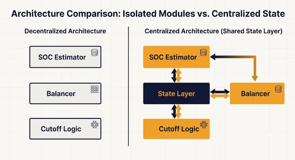
Most BMS designs treat SOC estimation, cell balancing, and cutoff protection as three separate modules. Each one runs its own logic. Each one reads its own inputs. This works, but it leaves value on the table. An integrated BMS control architecture ties these three functions together instead. They share one live state, not three separate guesses. This guide covers what that shared state looks like, and why it matters for LFP. New to BMS fundamentals first? Our BMS explained guide covers the basics before returning here.
⚡ Quick Answer An integrated BMS control architecture means the SOC estimator, the cell balancer, and the cutoff logic all read from one shared, current view of each cell’s voltage, resistance, and temperature. Without this link, each subsystem can act on a slightly different picture of the pack, and small disagreements between them compound into real errors.
Why Three Separate Modules Create Hidden Errors
This challenge is related to a broader question in battery-pack monitoring: whether separately-run, local estimators can be trusted to agree with a fully centralized view. Research on distributed Kalman filtering across battery pack cells explores this tradeoff for thermal estimation specifically, finding that distributed approaches can track a centralized estimate closely when properly designed — the same coordination problem this article addresses for SOC, balancing, and cutoff logic. A BMS built as three separate modules seems simpler at first. But each module often keeps its own internal estimate of pack state. The estimator has its own SOC value. The balancer has its own view of cell voltage spread. The cutoff logic has its own read on present resistance. These three views should agree. In practice, small timing gaps and separate filtering choices let them drift apart, even by a small amount.
A Concrete Example of the Problem
Picture a cell under a sudden high-current pulse. The estimator’s filter may lag the true voltage sag. The lag can run a few hundred milliseconds. The cutoff logic reads raw current and voltage directly. So it reacts faster. It might trip a cutoff. The estimator’s own SOC value says this should not happen yet. Without shared state, this looks like a bug. An integrated BMS control architecture fixes it. Both systems read the same current-corrected voltage, in real time. The mismatch does not occur.
What Shared State Means for an Integrated BMS Control Architecture
An integrated BMS control architecture is not one giant algorithm. It is a shared data layer that each function reads from and writes to. At minimum, this layer holds present cell voltage, present current, present temperature, the estimator’s current SOC output, and the present DCIR value drawn from the resistance lookup table. Every subsystem calculates from this same set of numbers, on the same update cycle.
Update Timing Matters as Much as the Data Itself
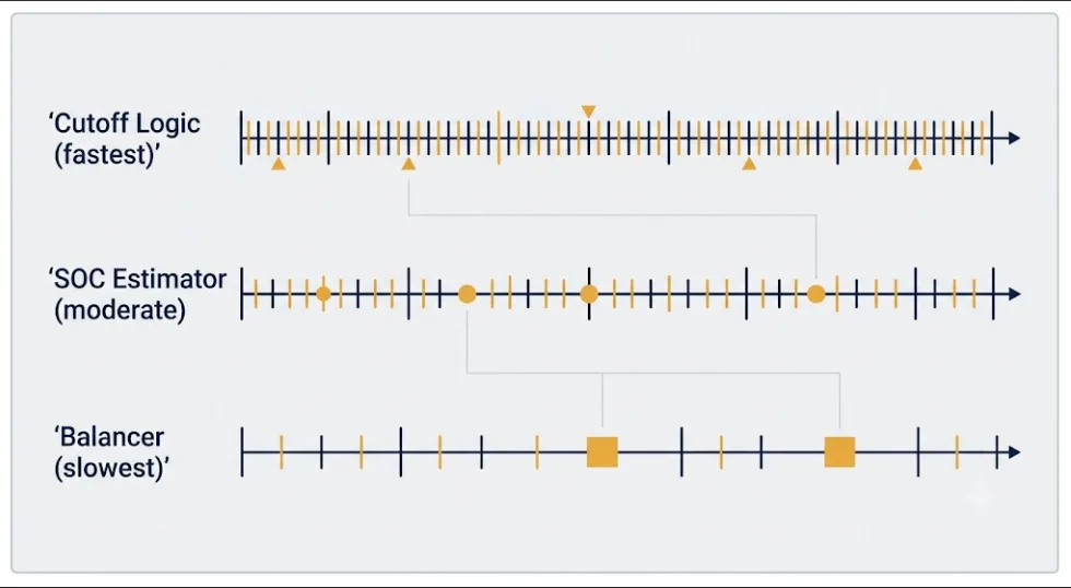
Sharing the right data at the wrong update rate still causes disagreement. The cutoff logic needs the fastest update path. A hard voltage limit can be reached in milliseconds, under a current spike. The SOC estimator can run on a slower cycle instead. Its correction task is inherently smoother. Design the shared state layer so each subsystem pulls at its own needed rate. Do not force one single rate onto all three.
How Subsystems Interact in an Integrated BMS Control Architecture
With shared state in place, the three subsystems can do more than avoid disagreement. They can actively support one another. The estimator’s SOC output can flag the balancer toward cells worth watching. The balancer’s voltage-spread data can flag the estimator when a cell’s behavior looks abnormal, rather than just imbalanced. The cutoff logic’s live DCIR reading, drawn from the same lookup table an EKF SOC estimation design pulls its resistance model from, keeps both systems working from one resistance picture instead of two.
Flagging Faults Instead of Silently Adapting
A well-built integrated BMS control architecture also creates a natural place to catch faults. If the shared DCIR reading from one cell departs sharply from its neighbors, and that departure does not track with the pack’s overall temperature or aging trend, the architecture can flag it as a possible fault, tied to the same in-service cell imbalance and DCIR drift patterns covered elsewhere in this series. This is far harder to catch when each subsystem only sees its own narrow slice of the picture.
Implementing an Integrated BMS Control Architecture Without a Full Redesign
For how centralized, modular, and wireless BMS topologies differ in where this shared layer can physically live, see our BMS architecture guide. Building an integrated BMS control architecture does not usually require new sensors. Most BMS hardware already measures voltage, current, and temperature at a resolution that supports this. The work is mostly in firmware: defining the shared data structure, setting update rates per subsystem, and routing each function’s calculation through the shared layer instead of an isolated local copy.
A Practical Migration Path
Start with the two subsystems most likely to disagree today: the SOC estimator and the cutoff logic, since both read current and voltage directly and both act on threshold logic. Confirm they draw from one shared, current-corrected voltage value before adding the balancer into the same layer. This staged approach limits the scope of any one firmware change and makes each step easier to validate on its own.
Key Takeaways
Three separate BMS modules can quietly disagree, even when each one works correctly on its own. An integrated BMS control architecture fixes this with one shared data layer for voltage, current, temperature, SOC, and DCIR, read by all three subsystems. Update timing matters as much as the shared data itself; each subsystem should pull at the rate its own task needs. Shared state also creates a natural place to flag developing faults, since a real fault shows up as one cell’s data breaking pattern against the rest of the shared picture.
Frequently Asked Questions
Does an integrated BMS control architecture need new hardware?
Usually not. Most BMS hardware already measures voltage, current, and temperature at a fine enough resolution. The work is mainly firmware: building a shared data layer and routing each subsystem’s calculation through it.
Which two subsystems should be integrated first?
Start with the SOC estimator and the cutoff logic. Both read current and voltage directly, and mismatches between them are the most likely to show up as a false or late cutoff trip.
How does an integrated BMS control architecture help catch developing faults?
When every subsystem shares one live view of each cell, a real fault shows up as that cell’s data breaking pattern against its neighbors and against the pack’s overall trend, rather than being missed by a subsystem that only sees its own narrow slice of the picture.
Cell matching before pack assembly sets a good starting point. But it does not stay good forever. In-service cell imbalance builds up over years. It builds long after the pack leaves the factory well matched. Heat, aging, and cycling all pull cells apart again. This guide covers the design choices that slow that drift. It covers thermal layout, balancing topology, and how imbalance control ties back into SOC estimation.
⚡ Quick Answer In-service cell imbalance grows mainly from two sources after assembly: uneven pack temperature, and the uneven aging that follows from it. Good thermal design and the right balancing topology both slow this drift. Neither one fixes a pack that started out badly matched.
Why In-Service Cell Imbalance Differs from Factory Mismatch
Factory cell matching solves the starting-point problem. Our cell matching before pack assembly guide covers that stage in depth. It groups cells by voltage, capacity, and resistance before assembly. In-service cell imbalance is a different, ongoing problem, however, because even a well-matched pack drifts apart over time. The BMS balances small gaps every cycle. But the size of that gap depends on design choices made outside the BMS itself.
The Feedback Loop Between Heat and Aging
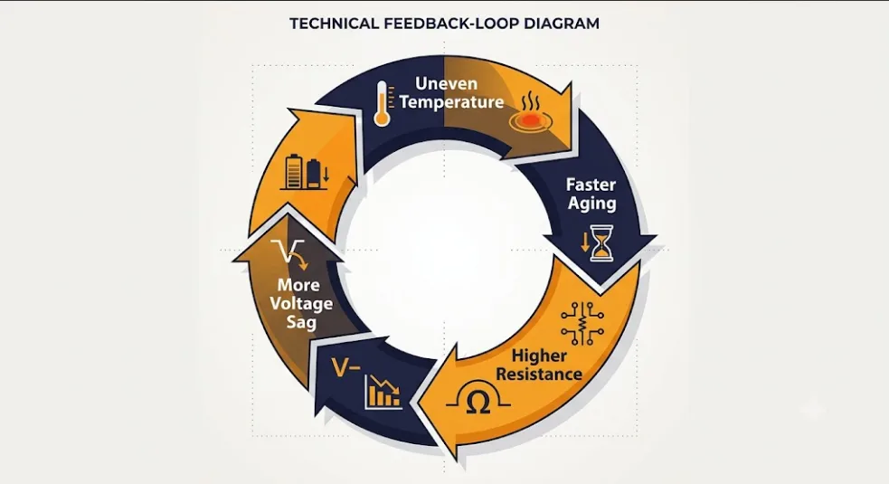
This pattern matches published research on thermal gradients in lithium-ion packs, which found that uneven internal temperature drives inhomogeneous degradation and resistance growth well before a pack reaches end of life on paper. Heat is the main driver of in-service cell imbalance. A cell that runs hotter than its neighbors ages faster. It loses capacity faster and, as a result, it gains resistance faster too. Consequently, that resistance rise makes it sag more under load. More sag can make it run hotter still, at the same current. This is a feedback loop. Left unmanaged, a small temperature gap can grow into a real capacity gap. This can happen within a few years of daily cycling.
Designing Thermal Layout to Limit Imbalance
Thermal design is the first lever against in-service cell imbalance. It acts before the BMS ever needs to balance anything. For the specific causes of uneven pack temperature — coolant path position, cell position within the rack, and current-path resistance — and the ΔT targets a well-designed system should hit, see our cell temperature gradients guide. The takeaway for imbalance control specifically: any gradient beyond those targets does not just cost efficiency. It feeds directly into the heat-aging-resistance loop above, and the wider the gradient, the faster the affected cells pull away from the rest of the pack.
Design Around the Worst Case, Not the Average
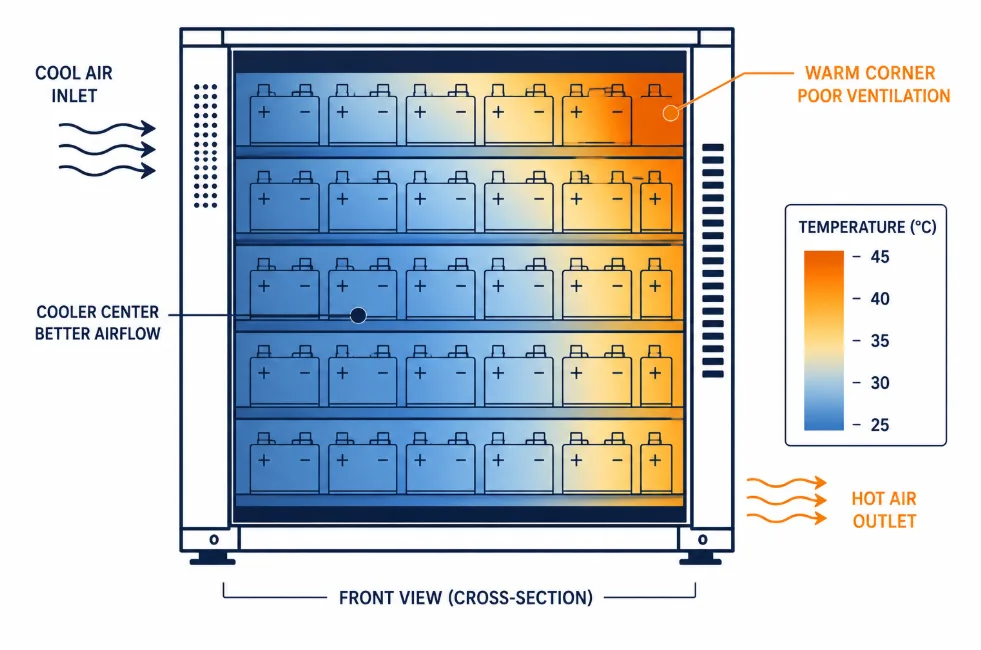
A common mistake sizes cooling around the pack’s average temperature. Average temperature can look fine. Meanwhile, individual cells can sit well outside it. Measure the worst-case gradient across the pack instead of the mean. Design cooling around that number. This resistance rise is the same mechanism covered in our cell internal resistance guide. A pack running meaningfully above those ΔT targets — commonly the case in a poorly ventilated rack corner — is exactly the failure mode that accelerates in-service cell imbalance in the affected cells, over a multi-year service life.
Choosing a Balancing Topology for the Cycling Profile
Balancing topology is the second lever. Passive balancing bleeds excess energy off higher-SOC cells as heat. It is simple and low-cost. It works fine for light daily cycling with well-matched cells. But passive current is small. It is often just tens to a few hundred milliamps. It cannot keep pace with fast-building imbalance under heavy cycling or a strong thermal gradient.
Feature
Passive Balancing
Active Balancing
Typical current
Tens to a few hundred mA
1–5A
Cost
Low
Higher, more hardware
Best fit
Light daily cycling, well-matched cells
Heavy cycling, thermal gradients, long-duration assets
Energy handling
Bleeds excess as heat
Moves energy between cells
Effect on in-service cell imbalance
Slows drift on light-use systems
Keeps pace with faster-building drift
When Active Balancing Earns Its Cost Against In-Service Cell Imbalance
Active balancing moves energy between cells instead of burning it off. It corrects gaps far faster, at one to several amps. This higher cost pays off in three cases. First, systems that cycle more than once daily, since imbalance gets less rest time between corrections. Second, systems with a thermal gradient that design alone cannot remove — the same resistance growth this drives also affects cutoff timing; see our DCIR-adaptive cutoff guide. Third, long-duration systems built for fifteen years or more, where small ongoing gains add up to real lifetime value.
Linking Imbalance Back to SOC Estimation
In-service cell imbalance and SOC estimation accuracy feed each other. A design that treats them as separate problems will underperform. A biased SOC estimate can send the balancer a false signal. It might correct a gap that is not really there. Or it might miss one that is. This is the same shared-state problem seen in EKF SOC estimation design. The balancer and the estimator both need one current, shared view of each cell. They should not run on two readings that can quietly disagree.
Setting a Practical Alert Threshold
A voltage spread over 50 to 100 millivolts across cells is a common alert threshold on LFP. The chemistry’s flat curve means even a real SOC gap may show only a small voltage difference. Log these events instead of reacting to one reading. A single high-current moment can cause a spread that resolves on its own.
Key Takeaways
In-service cell imbalance differs from factory cell matching. It is driven mainly by heat, and the aging that heat speeds up. Thermal layout is the first line of defense, especially sizing cooling around worst-case gradients, not pack averages. Balancing topology should match the cycling profile. Passive balancing suits light daily cycling. Active balancing earns its cost in heavy-cycling, high-gradient, or long-duration systems. Imbalance control and SOC estimation should share state, not run as separate systems, since each one affects the accuracy of the other.
Frequently Asked Questions
What causes in-service cell imbalance if the pack started well matched?
Uneven pack temperature is the main driver. Hotter cells age faster and gain resistance faster. That raises sag under load, which can push the cell hotter still. The gap compounds over years of cycling.
Does active balancing fix a pack that started out mismatched?
No. Active balancing corrects ongoing in-service cell imbalance much faster than passive balancing. But neither approach can create capacity a weak cell never had. A bad starting mismatch still needs fixing at the cell-matching stage, before assembly.
What voltage spread signals a real in-service cell imbalance problem on LFP?
A spread over 50 to 100 millivolts is a common threshold worth checking. Still, the trend across cycles matters more than any single reading.
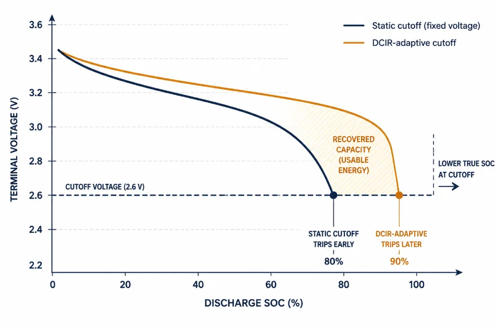
A static low-voltage cutoff pulls one fixed value from a cell datasheet. That single number is one of the most common reasons a BESS underdelivers its rated usable capacity. As direct current internal resistance (DCIR) rises with cell age, it also rises as temperature drops. The voltage sag under load grows along with it. A fixed cutoff trips earlier and earlier in the discharge curve, even though the cell still has real, recoverable capacity left. This article walks through how to design a DCIR-adaptive cutoff instead. It covers the test data it requires, the lookup-table structure a BMS actually implements, and the throughput recovered as a result.
⚡ Quick Answer A DCIR-adaptive cutoff replaces one fixed trip voltage with a value calculated in real time. It pulls current and a resistance value from an HPPC-derived lookup table, indexed by SOC, temperature, and cell age. This raises the effective cutoff trigger to match present-moment resistance, instead of a fresh-cell assumption — recovering up to 10% of effective throughput in mid-to-late project life that a static cutoff would otherwise strand.
Why a Fixed Cutoff Voltage Is the Wrong Design Choice
A discharge cutoff exists to stop the pack before any cell drops below its safe minimum voltage — commonly 2.5V per cell for LFP. The problem is where that voltage gets measured. Terminal voltage under load equals open-circuit voltage minus the resistive sag: V(terminal) = V(OCV) − I × DCIR. A fresh cell with 0.15 mΩ DCIR sags very little even at high current. The same cell after several thousand cycles sags far more. Its DCIR has risen to 0.3–0.5 mΩ, and it sags two to three times as much at identical current. So the BMS reaches the 2.5V trip point at a meaningfully higher residual state of charge, even though the cell’s actual OCV-based SOC has not changed.
Temperature compounds this effect further. Internal resistance rises sharply as cell temperature falls. Ion mobility slows down in the cold, both in the electrolyte and at the electrode interface. A cutoff threshold validated only at 25°C on a fresh cell will trip early on both counts, in a cold, aged pack. Sometimes this strands 10–15% of nameplate capacity that the cell was never actually short of.
Building the DCIR-SOC-Temperature Map for a DCIR-Adaptive Cutoff
The data foundation for a DCIR-adaptive cutoff is Hybrid Pulse Power Characterization (HPPC) testing. This methodology was developed under the US Department of Energy’s USABC/PNGV programs. It is now standard practice across automotive and stationary storage cell qualification. HPPC applies paired discharge and charge current pulses at fixed SOC steps, typically every 10% of capacity. It runs this across a matrix of test temperatures, and measures the resulting voltage response to extract resistance at each point. This is the same underlying test data an EKF SOC estimation design uses to build its own equivalent circuit model. A project running one HPPC campaign can feed both efforts from a single test matrix.
Discharge the cell to each target SOC step and allow it to rest until voltage stabilizes.
Apply a short current pulse (commonly 10 seconds) at the rated or peak discharge current and record the instantaneous voltage drop.
Calculate DCIR at that SOC and temperature as ΔV divided by the pulse current.
Repeat across the full SOC range and across a temperature matrix spanning the system’s expected operating envelope, from cold-climate minimums to peak ambient.
Repeat the full test periodically through a cycle-aging program to capture how the resistance surface shifts with cell age, not just with SOC and temperature.
The output is a three-dimensional resistance surface — DCIR as a function of SOC, temperature, and cycle count or SOH — rather than a single number. This surface is what the BMS firmware references at runtime instead of a fixed cutoff voltage.
From Resistance Surface to a DCIR-Adaptive Cutoff Lookup Table
Translating HPPC data into a working DCIR-adaptive cutoff requires converting the continuous resistance surface into a discrete lookup table. This table has to be one the firmware can query in real time, without heavy onboard computation.
Structuring the Lookup Table
A practical implementation follows this structure:
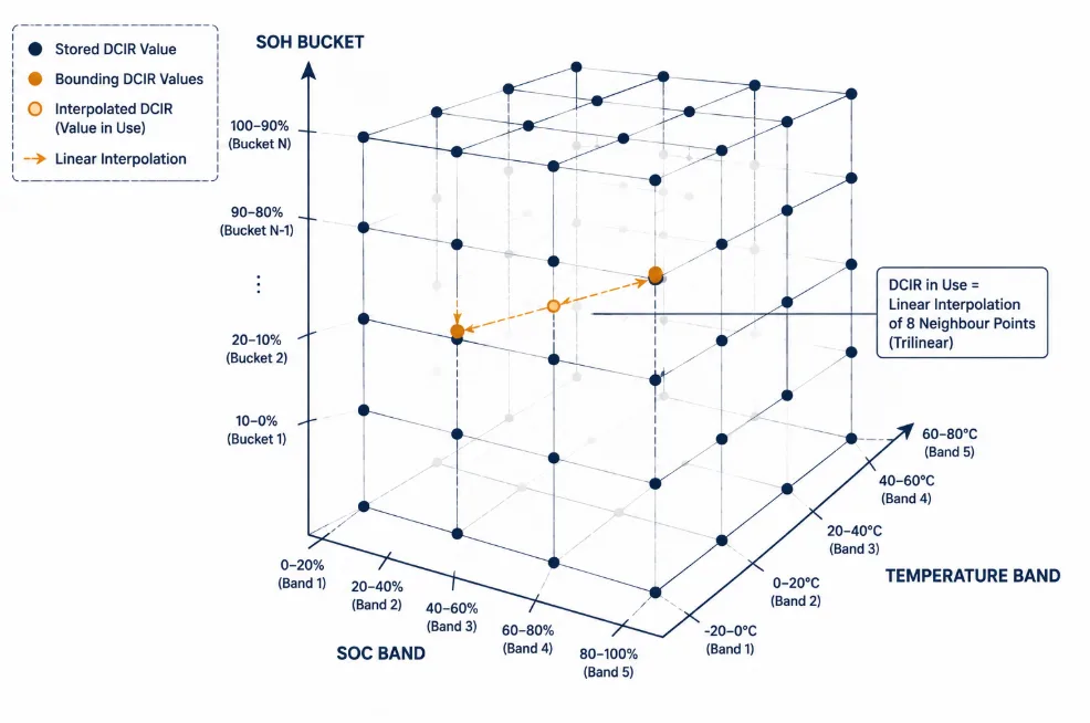
Index the table by SOC band (e.g., 10% steps), temperature band (e.g., 5°C steps), and a coarse SOH bucket (e.g., every 500–1,000 cycles or a measured capacity-fade threshold).
Store a DCIR value at each grid point, interpolating linearly between points at runtime rather than storing every possible combination.
Calculate the adjusted cutoff voltage in real time as V(cutoff, adjusted) = V(cutoff, minimum) + I(measured) × DCIR(SOC, T, SOH) — raising the effective cutoff trigger point to reflect present-moment resistance rather than a static assumption.
Apply hysteresis around the cutoff transition to prevent the BMS from oscillating between discharge-enabled and discharge-disabled states as current and resistance fluctuate near the boundary.
Re-anchor the SOH bucket periodically using either a full capacity test or a DCIR-trend proxy, since resistance growth is one of the standard leading indicators for SOH estimation without requiring a full discharge test.
Using resistance trend as an SOH proxy rather than running a full capacity test lines up with current battery-health research: a recent review of experimental health-assessment methods for lithium-ion cells names pulse-based resistance testing among the practical indicators for tracking degradation without the time and equipment cost of a full discharge cycle.
How Static and DCIR-Adaptive Cutoffs Compare
Reference point
Single fixed voltage from cell datasheet
Real-time calculated voltage adjusted for measured current × DCIR
Temperature handling
Assumes room-temperature test conditions
Indexed by temperature band from HPPC matrix
Aging handling
Fixed for asset life
Indexed by SOH bucket; re-anchored periodically
Typical result at 1C, mid-to-late project life
10–15% of nameplate capacity stranded
Recovers up to 10% of effective throughput
Data source
Cell datasheet single-point spec
HPPC test matrix across SOC × temperature × cycle count
Where the Recovered Throughput Comes From
The revenue case for this design change is straightforward. DCIR-driven voltage sag can shrink the usable SOC window by roughly 10–15% in mid-to-late project life, at high C-rates. Our 0.5C vs 1C cycle life analysis puts a number on the recoverable share of that: a DCIR-adaptive cutoff recovers up to 10% of effective throughput in mid-to-late project life. It does this by letting discharge continue closer to the cell’s true low-SOC limit, rather than tripping on resistance alone. Over a multi-year asset life, this compounds. Every cycle that discharges 10% deeper than a static cutoff would have allowed is 10% more throughput on that cycle. Multiply that across thousands of cycles. For dispatch-contracted or market-facing assets, this also improves bid accuracy. The state-of-charge and state-of-power figures reported to the EMS more closely match what the pack can actually deliver under load.
Implementation Notes and Common Pitfalls
Don’t confuse SOC estimation with cutoff calibration
A DCIR-adaptive cutoff corrects for resistance-driven voltage sag; it does not replace the underlying SOC estimation algorithm. An accurate EKF-based SOC estimate can still trip early under load if the cutoff voltage itself is static. Both layers need attention. For the estimation side of this problem, including how a biased SOC output can itself shift where a DCIR-adaptive cutoff trips, see our EKF SOC estimation design guide. SOC estimation accuracy and cutoff voltage adaptivity solve different problems that happen to share the same root cause in LFP’s flat OCV curve.
Validate That the DCIR-Adaptive Cutoff Doesn’t Mask Genuine Cell Faults
A DCIR-adaptive cutoff must still tell apart two different things. One is normal, predictable resistance growth. The other is an abnormal resistance spike from a developing fault — a loose busbar connection, a failing weld, or accelerated local aging tied to in-service cell imbalance. Cross-check measured DCIR against the expected value from the lookup table, rather than blindly applying the adjustment. This lets the BMS flag anomalies instead of quietly adapting around them.
Size cooling and current limits around end-of-life DCIR, not fresh-cell DCIR
The same resistance surface that feeds the cutoff table should also inform thermal design margin and current-limiting logic. Heat generation scales with resistance and the square of current. Designing cooling capacity around fresh-cell impedance under-sizes the system for the DCIR it will actually see in year eight or ten. None of these three systems — cutoff logic, SOC estimation, and imbalance control — should run as fully isolated modules. Our integrated BMS control architecture guide covers how to share DCIR, current, and temperature state across all three.
Key Takeaways
A fixed low-voltage cutoff ignores the fact that DCIR rises with both cell age and cold temperature, which strands usable capacity that the pack technically still has. HPPC testing across a SOC × temperature × cycle-count matrix is the standard method for building the resistance data a DCIR-adaptive cutoff needs. The firmware implementation is a lookup table with linear interpolation, not a continuous real-time model — this keeps the calculation lightweight enough for BMS hardware. A DCIR-adaptive cutoff recovers up to 10% of effective throughput in mid-to-late project life, most of the capacity that would otherwise sit stranded behind a static, resistance-blind trip point. Cutoff adaptivity and SOC estimation accuracy are separate problems. Both trace back to LFP’s flat voltage curve. Fixing one does not fix the other.
Frequently Asked Questions
Is a DCIR-adaptive cutoff a firmware-only change, or does it require new hardware?
In most cases it is a firmware and calibration-data change rather than a hardware change, provided the BMS already measures cell voltage and pack current with sufficient resolution and sampling rate. The work is in generating the HPPC-derived lookup table and implementing the interpolation and hysteresis logic, not in adding sensors.
How often does the resistance lookup table need to be re-validated?
A practical cadence ties re-validation to SOH milestones rather than a fixed calendar interval — for example, every 500–1,000 cycles or whenever a capacity or DCIR trend crosses a defined threshold. Systems with continuous DCIR trending can trigger table updates automatically rather than requiring a manual test campaign.
Does a DCIR-adaptive cutoff increase the risk of over-discharging a cell?
No, when implemented correctly. The adjustment raises the effective cutoff trigger voltage to compensate for load-induced sag. It does not lower the cell’s true minimum safe voltage. That real, OCV-based SOC is still where the cell trips. The BMS is simply better at recognizing where that point is under load, instead of confusing resistive sag for depleted charge.
References
• HPPC Test Procedure — Hybrid Pulse Power Characterisation methodology originating from the USABC/PNGV development program.
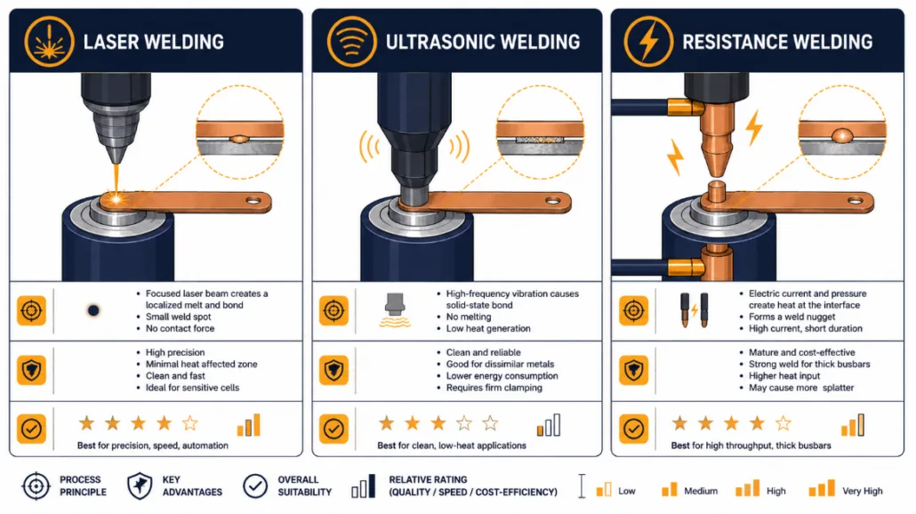
⚡ Quick Answer: Which Busbar Welding Method Is Best? Battery pack busbar welding uses three main methods: laser, ultrasonic, and resistance welding. Overall, laser welding gives the strongest, lowest-resistance joint and suits high-current packs. By contrast, ultrasonic welding avoids melting the metal, which makes it a strong fit for thin foils and aluminum. Resistance welding costs less to set up, but it tolerates dissimilar, highly conductive metals less well at scale. Ultimately, the right choice depends on your busbar material, current load, and production volume.
Battery pack busbar welding turns individual cells into an electrically connected string. Every joint in that string carries real current, often 200 amps or more in a BESS pack. A single weak weld raises resistance at exactly the point where the pack can least afford it.
Peer-reviewed research on tab-to-busbar joints backs this up. One study in the journal Batteries found that resistance and temperature rise at a weld joint varied by material choice and weld parameters. In short, busbar welding is not a cosmetic step. Instead, it is an engineering decision with real safety and performance consequences. Below, the sections cover busbar types first, then compare the three welding methods manufacturers actually use.
2. Types of Battery Pack Busbars: Material, Size, and Thickness
Copper vs. Aluminum: The Core Material Choice
Busbar choice starts with the metal. Copper carries current more efficiently than aluminum. As a result, a copper busbar can run thinner than an aluminum busbar rated for the same current. A 300A pack, for example, might use a 3mm-thick copper bar. An aluminum bar for the same job would need to be about 5mm thick.
However, aluminum costs less. It also weighs about half as much as copper at equal current rating. That is why some large-format packs use it despite the bulkier cross-section. On the other hand, aluminum forms a natural oxide layer that raises joint resistance if it is not managed. This is one reason ultrasonic welding, which does not melt the metal, pairs well with aluminum busbars.
Why Nickel-Plated Copper Is Standard for Lithium Packs
For lithium battery packs specifically, nickel-plated copper is the most common busbar choice. The nickel layer resists corrosion. It also helps the busbar hold a stable, low resistance across thousands of thermal cycles. Because copper melts predictably under a controlled beam, nickel-plated copper busbars suit laser welding well. In addition, they weld cleanly with ultrasonic methods on thinner gauges. Overall, this material choice is one of the first decisions in any battery pack busbar welding project.
Matching Busbar Thickness to the Battery Pack Busbar Welding Method
Thickness follows current, not cell format. Many LiFePO4 prismatic cells use busbars around 25mm wide. Their thickness scales with the amperage the joint has to carry. Generally, thin busbars under roughly 3mm favor ultrasonic welding, since there is little material to melt safely. By contrast, thicker busbars above 3mm favor laser or resistance welding, since they can absorb more heat without damage. Getting this pairing right is a core part of planning battery pack busbar welding before production starts.
Overall, the table below summarizes how material and thickness map to welding method.
Busbar Type
Typical Thickness
Best Welding Match
Why
Bare or tinned copper
2-6 mm
Laser or resistance
Best conductivity; carries high current in a thin profile
Nickel-plated copper
2-5 mm
Laser or ultrasonic
Standard for lithium packs; corrosion resistance plus a stable, low-resistance weld
Aluminum
4-10 mm
Ultrasonic
Needs a larger cross-section; oxide layer favors a non-melting method
Copper-aluminum transition
Varies
Specialized ultrasonic or bonded
Prevents galvanic corrosion where dissimilar metals meet
3. Laser Welding for Battery Pack Busbars
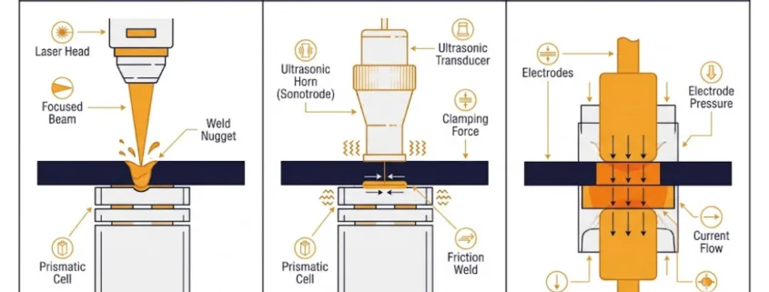
Laser welding uses a focused, high-energy beam to melt and fuse the busbar to the cell terminal. The joined metal resolidifies almost instantly. As a result, there is very little time for oxygen or contaminants to weaken the weld.
Overall, this method produces deep, strong joints, sometimes reaching close to the strength of the base metal. It also creates a smaller weld spot than ultrasonic welding, which allows tighter cell packing. However, laser systems cost more upfront. In addition, the process needs tight control over spot size, power, and scan speed, since a poorly tuned laser can damage nearby cells.
4. Ultrasonic Welding for Battery Pack Busbars
Ultrasonic welding joins metal without melting it. Instead, mechanical vibration creates friction at the joint, bonding the surfaces together. Because there is no melting involved, the heat-affected zone stays small, which protects nearby cells and thin materials.
Consequently, this makes ultrasonic welding a common choice for aluminum busbars and thin foils, where excess heat could easily cause damage. However, the tradeoff is that the bond mostly occurs at the surface, with limited penetration into the material. For very high current paths, manufacturers sometimes need multiple ultrasonic joints where a single laser weld would do the job.
5. Resistance Welding for Battery Pack Busbars
Resistance welding passes a high current through the joint, and the resulting heat fuses the metal together. It is the simplest and least expensive of the three methods. Therefore, some lower-volume or cost-sensitive lines still use it.
That said, resistance welding tolerates dissimilar, highly conductive materials less well at scale. It also generally produces more spatter than laser or ultrasonic methods. For high-reliability BESS packs, most manufacturers reserve resistance welding for less current-critical connections rather than the main busbar string.
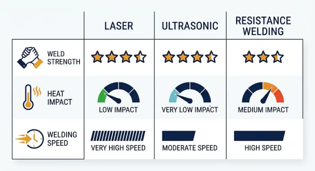
6. Laser vs Ultrasonic vs Resistance Welding: A Side-by-Side Comparison
Overall, the table below summarizes how the three methods stack up on the factors that matter most for battery pack busbar welding.
Factor
Laser
Ultrasonic
Resistance
Joint strength
Up to ~90% of base metal
85-95% conductivity, surface bond
Moderate, material-dependent
Heat impact
Low, tightly controlled
Very low, no melting
Higher, more spatter risk
Typical speed
~50 ms per joint
~100 ms per joint
Fast, but less precise
Best material fit
Copper, nickel
Aluminum, thin foils
Similar, conductive metals
Equipment cost
High
Moderate
Low
7. How Manufacturers Verify Battery Pack Busbar Welding Quality
A weld can look clean and still carry too much resistance. That is why pull-force testing happens right after welding on most production lines. This check confirms that each joint meets a minimum mechanical strength standard before the pack moves forward.
Many manufacturers also retest DCIR after welding, since resistance mismatches introduced at this stage become measurable immediately. In addition, some lines add X-ray inspection or cross-section sampling on a batch basis. This checks weld penetration depth directly, rather than relying on surface appearance alone.
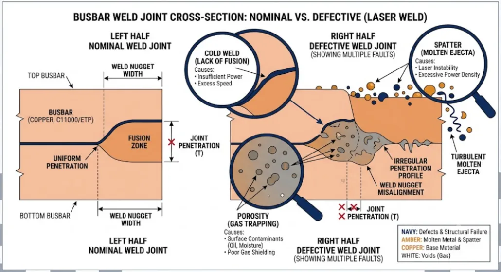
8. Common Busbar Welding Defects and What They Cause
Generally, these defects trace back to one of four causes on the production line.
Cold welds: too little heat or energy reaches the joint, leaving high resistance behind a surface that still looks connected.
Spatter contamination: molten particles land on nearby cells or contacts, risking short circuits or corrosion over time.
Porosity and voids: trapped gas weakens the joint internally, even when the surface passes a visual check.
Misalignment: a poorly stacked module (see our module stacking guide) creates weld gaps before the welding stage even begins.
9. Questions to Ask About a Manufacturer’s Battery Pack Busbar Welding Process
Which welding method do you use for busbars, and why did you choose it for this product?
What busbar material and thickness do you use, and how did you size it for our current rating?
What pull-force or peel-strength standard does every weld have to meet?
Do you retest DCIR after welding, and can you share that data for our batch?
How do you inspect for spatter contamination and porosity, and how often?
Conclusion: Battery Pack Busbar Welding Sets the Electrical Backbone of the Pack
Every welding method involves tradeoffs. Laser welding offers strength and low resistance, at a higher equipment cost. Meanwhile, ultrasonic welding protects heat-sensitive materials, but needs more joints for high current. By contrast, resistance welding costs less, but performs worse on dissimilar, highly conductive metals.
Ultimately, no single method is right for every product. What matters is whether a manufacturer chose their method deliberately. It also matters whether they can prove weld quality with real test data. That, in the end, is the real signal of a controlled battery pack busbar welding process, not the method name on a spec sheet.
☀️ Evaluating a Pack Supplier’s Weld Quality? Sunlith Energy reviews welding QC records, pull-force data, and DCIR retest results for BESS projects from 50 kWh upward. Contact us before you finalize a pack supplier.
Method Comparison at a Glance
Method
Best For
Watch Out For
Laser Welding
High-current packs needing deep, strong joints
Higher equipment cost, needs tight process control
Ultrasonic Welding
Thin foils, aluminum, low heat-affected zone
Surface-only bond, more joints for high current
Resistance Welding
Lower-cost, simpler production lines
Struggles with dissimilar, highly conductive metals
Frequently Asked Questions About Battery Pack Busbar Welding
What metal is best for a battery pack busbar?
It depends on the application. Copper carries the most current for its thickness, which suits high-current BESS packs. However, aluminum costs less and weighs less, though it needs a larger cross-section for the same current. Overall, nickel-plated copper is the most common choice for lithium packs, since it resists corrosion and welds well.
What is the best welding method for battery pack busbars?
There is no single best method. Instead, laser welding suits high-current packs that need deep, strong joints. Ultrasonic welding, meanwhile, suits thin foils and aluminum, where low heat matters most. Resistance welding fits lower-cost lines joining similar, conductive metals.
Why does battery pack busbar welding matter for safety?
A poor weld raises resistance at the joint. As a result, higher resistance means more heat under load. Over time, that heat can age one section of the pack faster than the rest. In the worst case, a weak joint can fail outright and create a safety event.
How do manufacturers test busbar weld quality?
Most run a pull-force test right after welding, since a joint that looks fine can still carry too much resistance. In addition, many also retest DCIR after welding. Some lines add X-ray or cross-section sampling to check penetration depth on a batch basis.
Is laser welding always better than ultrasonic welding?
Not always. Laser welding generally produces a stronger, lower-resistance joint. However, ultrasonic welding avoids melting the metal entirely, which some manufacturers prefer for thin or heat-sensitive materials. Ultimately, the right choice depends on the busbar material and current load.
What causes a cold weld in battery pack busbar welding?
A cold weld happens when the process delivers too little heat or energy to fully fuse the joint. In addition, contamination, surface oxidation, and misaligned parts can all contribute. The result is a joint that looks connected but carries far more resistance than it should.
Should I ask my battery pack supplier about their welding process?
Yes. Specifically, ask which welding method they use and what pull-force standard they test to. Also ask whether they can share weld QC data for your batch. Overall, a supplier who answers clearly is usually running a controlled battery pack busbar welding process, not just an assembly line.
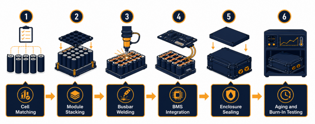
⚡ Quick Answer: What Is the Battery Pack Assembly Process? The battery pack assembly process turns screened cells into a finished, protected energy storage unit. It moves through six stages: cell sorting and matching, module stacking and compression, busbar welding, BMS integration, enclosure sealing, and aging or burn-in testing. Each stage sets a ceiling that later stages can’t fully recover from. A pack that skips or rushes an early stage rarely fails outright. Instead, it simply delivers less capacity and a shorter cycle life than its datasheet promised.
1. Why the Battery Pack Assembly Process Is a Manufacturing Discipline, Not a Wiring Job
Building a battery pack looks simple from the outside. You connect a group of cells, add a control board, and close the case. In practice, however, the battery pack assembly process works more like precision manufacturing than basic wiring. Small tolerances stack up at every stage. A cold weld here and an uneven compression force there can add up fast. As a result, the finished pack can fall short of the capacity and cycle life its datasheet promised.
This gap matters more for a BESS than for a small consumer device. That’s because a stationary pack runs thousands of cycles over 10 to 20 years. In fact, international safety standards such as IEC 62619 exist precisely because assembly quality drives real-world safety, not just performance. For a broader view of how pack assembly fits within a complete system, read our guide to key components in a BESS architecture. Below, the sections walk through each stage in the order it happens on a production line.
2. Stage 1 of the Battery Pack Assembly Process: Cell Sorting and Matching
Before a single cell reaches the assembly line, workers sort it by voltage, capacity, and internal resistance. Even cells from the same production batch vary slightly. Therefore, grouping similar cells together reduces how much correcting the BMS has to do later. Typically, manufacturers run a fast ACIR screen first, then confirm with DCIR pulse testing before final grouping.
For a full breakdown of this step, read our complete cell matching before pack assembly guide. It covers how internal resistance affects series versus parallel groups. In short, this is the foundation stage of the entire battery pack assembly process. Every later stage inherits whatever variation this one leaves behind.
3. Stage 2: Module Stacking and Mechanical Compression
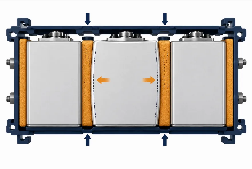
Once cells are sorted, they move into module stacking. End plates and pressure plates apply a controlled compression force across the stack. This keeps prismatic and pouch cells in steady contact. It also leaves room for the swelling that naturally happens over a cell’s charge cycle. Before this step locks in, a CCD vision system checks tab and terminal alignment. A misaligned cell here creates a welding problem two stages later.
Adhesives also enter the process at this stage, and they do two separate jobs. On one hand, a compliant thermal interface material carries heat away from the cells. On the other, a smaller, targeted structural adhesive bead helps hold the stack together, without resisting the swelling that compression plates already accommodate. Our guide to gluing cells in a battery pack covers which adhesive chemistry fits which job. It also explains why a rigid, full-face bond causes many long-term pack failures.
Afterward, steel straps or plastic-steel banding secure the stack for transport to the welding station. Bottom flatness matters here too, since an uneven module base creates gaps against thermal pads or cooling plates further downstream. Eventually, that gap shows up as an uneven temperature distribution, a problem we cover in our guide to cell temperature gradients in BESS.
4. Stage 3: Busbar Welding and Electrical Interconnection
Busbar welding turns individual cells into an electrically connected string. Three welding methods dominate this stage of the battery pack assembly process. First, laser welding offers high precision and low thermal impact. Meanwhile, ultrasonic welding works fast and handles dissimilar metals without melting either surface. By contrast, resistance welding is the simplest method, but it tolerates dissimilar, highly conductive materials less well at scale.
Right after welding, technicians verify weld quality with a pull-force test, since a joint that looks fine can still carry excessive resistance. For instance, a cold weld or particulate spatter left uncleaned can pierce a cell casing. It can also create a resistance hotspot, which then ages that section of the pack faster than the rest. Because this stage feeds directly into DCIR verification, any resistance mismatch becomes measurable before the pack moves forward.
5. Stage 4: BMS Integration and Wiring Harness
With the electrical interconnections complete, the battery management system goes in next. Technicians install cell supervision circuit (CSC) boards and connect sensor and communication wiring harnesses. In larger packs, they also wire multiple slave boards to a central master BMS. Because the busbars still sit at low voltage at this point, manufacturers deliberately install the BMS before final busbars bring the pack to full voltage. Consequently, this keeps the line safer for technicians.
6. Stage 5 of the Battery Pack Assembly Process: Enclosure Sealing and IP Rating
Once the BMS and wiring harness are in place, workers close the pack into its enclosure. They apply sealant, torque the lid to specification, and then run a leak-rate test to confirm the rated IP class. Generally, indoor commercial installs target IP65, while outdoor and utility-scale deployments exposed to rain, dust, or coastal humidity typically need IP66 or IP67.
At this stage, fire code compliance also starts to matter directly. Specifically, enclosure integrity, safety distances, and installation clearances feed into requirements covered under NFPA 855. Even so, a leak-tested but poorly torqued enclosure can pass an initial inspection and still fail years later, once gasket materials age and compress.
7. Stage 6: Aging, Burn-In, and Factory Acceptance Testing
The final stage of the battery pack assembly process is checking the work. First, the sealed pack goes through insulation resistance and withstand voltage testing. It then runs charge and discharge cycling that mirrors real operating conditions. Notably, this aging or burn-in period surfaces problems that earlier QC checks can miss. For example, a weak cell or a marginal weld connection can look fine under static testing. It may only reveal itself once the pack cycles under load.
For BESS-scale packs, this step overlaps with formal factory acceptance testing, which also verifies alarm thresholds, protection logic, and communication protocols before the pack ships. Our guide to BESS safety and compliance explains how factory-level testing connects to the certification requirements a finished system needs.
8. Cell-to-Pack vs Module-Based Assembly: A Quick Note on Architecture
Most of the stages above describe a module-based process: cells become modules, and modules become a pack. Alternatively, cell-to-pack (CTP) design skips the module step entirely and bonds cells directly to the pack structure and cooling plate instead. Because this removes an entire layer of module casings and interconnections, it can reduce weight, part count, and cost.
Still, the tradeoff is real. CTP removes the module-level buffer between a single bad cell and the whole pack. This places even more weight on the cell sorting and matching stage covered above. As a result, buyers evaluating a CTP-based product should ask harder questions about incoming cell grading. A module-based pack has more structural redundancy if a cell underperforms.
9. Quality Control Checkpoints in the Battery Pack Assembly Process
Overall, a well-run battery pack assembly process builds in a verification step after every major stage, not just at the very end. The table below summarizes what each checkpoint is designed to catch.
Stage
QC Checkpoint
What It Catches
Cell sorting
Voltage, capacity, DCIR/ACIR grading report
Mismatched cells before they ever reach a module
Module stacking
CCD alignment check, compression force verification
10. Questions to Ask a Manufacturer About Their Battery Pack Assembly Process
Do you test and match cells by voltage, capacity, and internal resistance before assembly?
Which busbar welding method do you use, and what pull-force standard do welds have to meet?
What IP rating does the sealed enclosure achieve, and is it leak-tested on every unit or by sample?
Do you run aging or burn-in cycles before shipment, and can you provide that data for our batch?
Is this a module-based or cell-to-pack design, and how does that affect your cell grading tolerance?
Conclusion: The Battery Pack Assembly Process Sets What the Finished Pack Can Deliver
Ultimately, no single stage of this process works in isolation. Cell matching sets the ceiling the BMS has to work within. Meanwhile, module compression and busbar welding determine how evenly that ceiling holds up over years of cycling. Finally, enclosure sealing and burn-in testing confirm, before the pack ships, whether earlier stages were done properly.
Therefore, when you evaluate a cell or pack supplier, ask about each stage specifically. Don’t just accept a general assurance that “the BMS handles it.” Instead, look for a manufacturer who can walk through their process stage by stage, with documentation at each checkpoint. That is what a genuinely controlled battery pack assembly process looks like, not a finished product with an unverifiable history.
☀️ Need Help Evaluating a Pack Manufacturer’s Assembly Process? Sunlith Energy reviews cell sorting data, weld QC records, enclosure test reports, and burn-in results for BESS projects from 50 kWh upward. Contact us before you finalize a cell or pack supplier.
Key Takeaways
Stage
What Happens
1. Cell Sorting & Matching
Workers grade cells by voltage, capacity, and internal resistance before assembly.
2. Module Stacking & Compression
Machines stack, compress, and mechanically retain cells to control swelling and vibration.
3. Busbar Welding
Laser, ultrasonic, or resistance welding connects cells in series and parallel.
4. BMS Integration
Technicians install and connect sensor wiring, CSC boards, and the master BMS.
5. Enclosure Sealing
Workers seal the pack to its rated IP class and leak-test it.
6. Aging & Burn-In Testing
Charge and discharge cycling, plus insulation tests, confirm the pack before shipment.
Frequently Asked Questions About the Battery Pack Assembly Process
What are the main stages of the battery pack assembly process?
Six stages make up the battery pack assembly process: cell sorting and matching, module stacking and compression, busbar welding, BMS integration, enclosure sealing, and aging or burn-in testing. Each stage builds on the one before it, so a defect introduced early is much harder to catch later.
Is battery pack assembly the same as cell manufacturing?
No. Cell manufacturing produces the individual lithium cells, tested and graded before they reach a pack line. By contrast, battery pack assembly starts once those finished cells arrive, and it covers sorting, stacking, welding, BMS integration, sealing, and testing. For the step that happens first, see our cell matching guide.
Why does battery pack assembly quality matter more for BESS than for a small consumer battery?
A stationary BESS pack runs thousands of cycles over 10 to 20 years, often at higher currents than a consumer device. Because of this, small defects that would go unnoticed in a phone battery compound over years of daily cycling. For example, a slightly cold weld or a poorly matched cell can turn into measurable capacity loss, or in the worst case, a safety event.
What is the difference between cell-to-pack and module-based assembly?
Module-based assembly groups cells into modules first, then combines modules into a pack. Cell-to-pack assembly, on the other hand, skips the module step and bonds cells directly to the pack structure. This can reduce weight and cost, but it also removes the module-level buffer between a bad cell and the full pack.
How long does battery pack assembly typically take?
For a utility-scale BESS pack, sorting, stacking, welding, and BMS integration can finish in hours on an automated line. However, aging and burn-in testing often adds one to several days, since full charge and discharge cycles take time but properly verify the pack before shipment.
What should I ask a manufacturer about their battery pack assembly process?
Ask which welding method they use for busbars, and whether they match cells before assembly. Also, find out what IP rating the enclosure achieves, and request burn-in test data for your specific batch. Overall, a manufacturer who answers all three with documentation is running a genuinely controlled battery pack assembly process.
Gluing cells is a normal step in battery pack assembly. Most modern packs use adhesive between the cells and the enclosure. However, gluing cells actually means two different jobs, not one. One material moves heat. Another material holds the pack together. Mixing up those two jobs is where most long-term problems start.
Quick Answer Gluing cells covers two different materials with opposite jobs. One is a soft, compressible thermal interface material (TIM) that carries heat away from cells. The other is a rigid structural adhesive that holds the pack together.Done correctly, gluing cells is safe and durable for the life of the pack. That means a controlled bond-line thickness, void-free contact, and room for swelling. Lithium cells swell 3–10% as they age.Done incorrectly, gluing cells can trap heat between cells. It can also crack under swelling stress. That happens when one adhesive covers both jobs, or when it’s spread across a cell’s full face with no room to expand.
Why Battery Packs Use Adhesives at All
Cell bonding didn’t replace bolts and brackets by accident. Pack designs moved from cell-module-pack layouts toward cell-to-pack and cell-to-chassis layouts. Adhesives took on jobs that used to need dozens of fasteners. For example, they join dissimilar materials such as steel, aluminum, and composite housings. A continuous bond line also damps vibration better than point contacts. In the most advanced designs, the cells themselves add stiffness to the enclosure. As a result, the pack becomes lighter, simpler, and often more energy-dense.
That shift is exactly why gluing cells deserves more scrutiny than it usually gets. One bond line now holds cells in place. It also moves heat. And it has to tolerate swelling, all at the same time. Consequently, getting the material or the process wrong causes one of three problems later: hot cells, cracked bonds, or a pack nobody can take apart.
The Two Jobs Behind Gluing Cells
Thermal interface materials and gap fillers
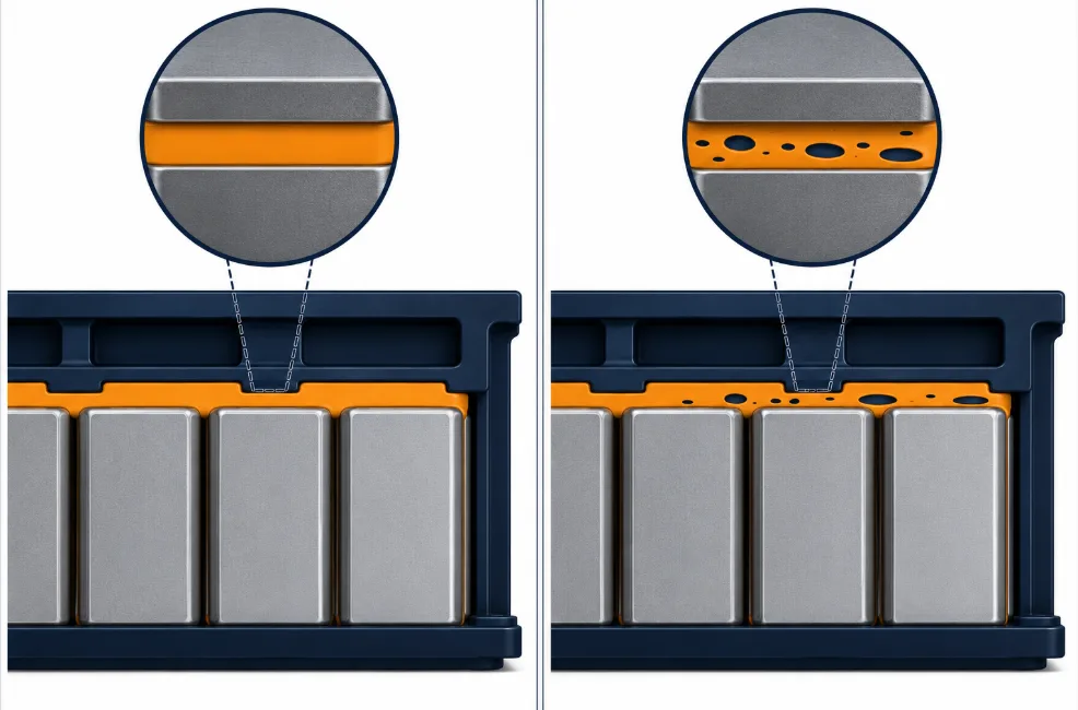
Thermal interface materials, or TIMs, are soft silicone or polyurethane pads, or dispensed pastes. They fill the microscopic air gaps between cells, modules, and cold plates. That gives heat a continuous path out, instead of an insulating air pocket. TIMs are built to be compliant, not strong. Gap fillers typically carry lap-shear strength below about 7 MPa. That’s far short of what’s needed to hold a cell in place. Their only job is heat transfer, so manufacturers keep them soft on purpose.
Structural adhesives used for gluing cells
Structural adhesives are the ones actually holding the pack together. They replace or support welds and fasteners. Epoxies bring high strength and chemical resistance. Toughened acrylics cure fast and resist peel and impact. Polyurethanes absorb vibration. They also tolerate the mismatched thermal expansion between metal housings and cell holders. A newer category, thermally conductive structural adhesive, tries to do both jobs in one material. That combination is a real trade-off, not a free upgrade. Pushing thermal conductivity up with more filler content tends to make the adhesive brittle. It also gets harder to dispense evenly.
How Gluing Cells Affects Heat Between Cells
Why an air gap traps heat
Every cell generates heat internally during charge and discharge. Neighboring cells in a tight module raise the stakes. Without a real thermal path between them, heat concentrates in the pack’s interior. It also builds up at poorly ventilated corners.
That’s the same mechanism behind the temperature spread covered in our guide to NMC vs. LFP thermal safety. For instance, a poorly managed corner of a rack can run 10–15°C hotter than the rest. The hottest cells age fastest. This isn’t a small effect — because degradation scales exponentially with temperature, not linearly, small gaps between cells compound rather than average out over years of service. See our guide on How Temperature Accelerates Battery Degradation: The Arrhenius Relationship for the mechanism behind why this matters so much. That pattern drags down the whole pack’s usable capacity, as covered in how temperature affects LiFePO4 cycle life.
An air gap between cells conducts heat poorly. So the material occupying that space does real thermal work, not just holding parts together. Displacing that air with a void-free, well-wetted TIM is what actually moves heat toward the cooling plate.
Why bond-line quality beats the datasheet number
Here’s the counterintuitive part: the conductivity number on a datasheet doesn’t predict real-world performance well. In one documented case, a 1.2 W/mK gap filler outperformed a 3.0 W/mK material at the pack level. The lower-conductivity material wet out the surfaces more completely. It also held consistent contact under compression. Meanwhile, a high-conductivity material applied with a thick or uneven bond line will underperform a lower-conductivity material applied well.
The same logic applies on the structural side. Structural adhesives usually conduct heat worse than purpose-built TIMs. A pack that relies on one universal adhesive for both jobs compromises on both. Separating the two zones keeps each material doing the job it was built for. Use a compliant TIM between cells and the cooling plate. Confine the structural bond to a smaller footprint, such as dots or beads, at the pack frame.
How Cell Swelling Affects Gluing Cells
Why cells swell
Lithium cells physically change volume as they cycle. Pouch and prismatic cells commonly swell 3–10% by volume as the graphite anode expands during normal charging. That swelling compounds with age. Gas generation and irreversible capacity fade set in over years of service. Therefore, a pack design that ignores this treats swelling as an afterthought, not a real load case.
The standard fix is mechanical, not adhesive. Compressible buffering elements sit between cells: gap pads, foam interlayers, or engineered compression pads. They accommodate expansion under a defined, controlled pressure over the pack’s full life. They also spread pressure more evenly across the stack. Engineers pick these materials for low creep and stable restitution. A pad that permanently deforms under years of cyclic compression stops doing its job long before the pack reaches end of life.
Why rigid gluing cells fails under swelling
This is where rigid gluing cells becomes a real failure mode. Picture a hard, fully cured structural adhesive spread across the whole face of a cell. Instead of accommodating expansion, it resists it. As the cell pushes against an unyielding bond line, stress concentrates at the casing and the electrode stack. The outcome can be casing deformation, internal delamination, or a cracked bond. That failure often happens at the exact moment good thermal contact matters most. It’s partly why engineers apply elastomeric adhesive as dots or beads instead of full-face coverage. A bead can stretch locally with the cell, instead of resisting it uniformly.
Is Gluing Cells Good for Long-Term Use, or a Problem?
Both, depending on how engineers design it. The honest answer isn’t a blanket yes or no.
What gluing cells gets right, long-term
Fewer parts and less weight than bolted or bracketed designs, without giving up structural stiffness
A continuous bond line damps vibration better than point-contact fasteners, cutting fatigue-driven loosening over years
A properly applied TIM closes the thermal gap that air leaves open, improving temperature uniformity rather than degrading it
Enables higher energy density cell-to-pack designs that frames and fasteners alone can’t match
Where gluing cells creates long-term liabilities
Disassembly for failure investigation or repair gets slow and hazardous. Teardown around cells sensitive to thermal runaway carries real risk
Some silicone-based TIMs outgas or migrate over years of thermal cycling. That’s why designers increasingly specify low-migration formulations near electrical contacts
A pack with no mechanical backup has no fallback. If a bond line degrades or disbonds from swelling stress over 10–15 years, nothing else holds the cell in place
Because of these trade-offs, the industry trend points toward keeping the benefits of gluing cells. At the same time, it builds in a path back out. That means adhesives designed for controlled debonding. It also means layouts that keep some mechanical retention as backup, instead of relying on the bond line alone.
Best Practices for Gluing Cells to Avoid These Problems
Separate the TIM zone from the structural zone
Don’t ask one adhesive to be both the heat path and the load path. Instead, use a compliant, thermally conductive gap filler between cells and the cooling plate. Confine structural bonding to a smaller footprint. Size it for the actual mechanical load, not the full cell face.
Control bond-line thickness
Specify and verify a controlled, thin, void-free bond line. Don’t just trust the conductivity number on a datasheet. A well-wetted, void-free interface at moderate conductivity consistently beats a high-conductivity material with air pockets or an uneven bond line.
Build swelling into the design, not just the adhesive
Treat swelling as its own load case. Use a compression pad with a defined force-deflection curve and low long-term creep. Don’t assume an adhesive bead will simply stretch forever. Where adhesive does touch cell faces, keep it in small, discrete beads. These can flex locally instead of forming one rigid full-face bond.
Match adhesive chemistry to the job
Epoxy: highest strength and chemical resistance, but rigid and brittle unless toughened. Use it where strength matters more than compliance
Acrylic: fast cure with good peel and impact resistance, which helps where production throughput matters
Polyurethane: absorbs vibration and tolerates thermal-expansion mismatch, often the better default for anything bonded directly to a cell
Silicone: highly compliant across a wide temperature range, the default for TIM pads and pastes. Confirm the formulation is low-migration near electrical contacts
Design for disassembly
Keep a mechanical fastening option at key access points where full structural bonding isn’t strictly required. Or specify a debonding-capable adhesive instead. This approach costs more up front. But it gives up little in performance. Over time, it turns a multi-hour, higher-risk teardown into a manageable service or recycling job.
Verify, don’t assume
Run pull tests. Inspect for voids with ultrasound or CT scanning. Use thermal imaging on prototype packs. These checks catch the gap between what a datasheet promises and what the dispensing process actually delivered. Bond-line quality is a process outcome, not just a material choice.
Key Takeaways on Gluing Cells
Question
Short Answer
Does gluing cells cause heat buildup?
Only with the wrong adhesive, voids, or a thick bond line. The right TIM lowers cell-to-cell temperature spread versus an air gap.
Does gluing cells survive swelling?
Rigid, full-face structural adhesive doesn’t. Compressible pads plus small adhesive beads do.
Can a pack with glued cells be repaired?
Harder than a bolted pack, but manageable with the right adhesive and access points designed in from the start.
Is gluing cells bad for long-term use?
Not inherently. The failures come from using one adhesive for every job, not from gluing cells itself.
Frequently Asked Questions About Gluing Cells
Does gluing cells make a battery pack run hotter?
Not with the right material in the right zone. A properly applied TIM displaces the air gap between cells and the cooling plate. That generally improves temperature uniformity compared with an unfilled air gap. However, heat buildup happens when a poorly conductive structural adhesive sits across a thermal path. It also happens when the TIM has voids or an uncontrolled bond-line thickness.
How much do cells actually swell?
Pouch and prismatic lithium cells commonly swell 3–10% in volume through normal cycling. Add more irreversible swelling as cells age and generate gas over years of service. As a result, pack mechanical design needs to treat this as a real load, not a rounding error.
Can a pack with glued cells be repaired or recycled?
Yes, but adhesive bonds are a well-documented obstacle. They make cell-level disassembly harder for repair, failure investigation, and direct recycling. That said, packs with debonding-capable adhesives or a mechanical backup are far easier to service and recycle than fully bonded designs with no fallback.
Is silicone or epoxy better for gluing cells?
They suit different jobs. Silicone is the default for compliant thermal pads and pastes, because it stays soft across a wide temperature range. Epoxy is stronger and more chemically resistant, which makes it common for structural bonding. Because epoxy stays rigid unless toughened, keep it away from surfaces that swell or flex.
Is mechanical fastening better than gluing cells?
Mechanical fastening allows easy disassembly. It also adds no cure-related risk. However, it typically has higher electrical resistance at the joint. It can loosen under vibration, and it adds bulk that works against energy density. Because of this, most modern packs mix both methods: fasteners or welds for electrical connections, and adhesive for thermal and structural bonding.
⚡ Quick Answer: What Is a Safe Temperature Gradient in a BESS Pack? A temperature gradient is the difference in temperature between the hottest and coolest cells in a pack at the same moment, often written as ΔT. Many BESS specifications target a maximum gradient of around 5°C across a rack, with premium liquid-cooled systems aiming closer to 2-3°C. A larger temperature gradient does not just mean one hot spot. It means cells are aging at different rates within the same pack, which widens the performance gap that cell matching worked to close in the first place.
1. Why Temperature Uniformity Is a Different Problem Than Cooling Capacity
Choosing between air and liquid cooling answers one question: how much heat can the system remove overall. It does not answer a second, separate question, however: does that heat leave every cell at the same rate? A BESS can have more than enough total cooling capacity. Even so, it can still run a large temperature gradient, if heat leaves some cells faster than others.
This distinction matters because gradient problems do not always show up as an overheating alarm. A pack can sit comfortably within its overall safe temperature range. Meanwhile, one corner of the rack quietly runs several degrees hotter than another, cycle after cycle. Nothing trips. Nothing alarms. The pack simply ages unevenly, and nobody notices until the SOH numbers start to diverge.
2. What Counts as a Safe Temperature Gradient
Exact gradient limits vary by manufacturer, cell chemistry, and system design. As a result, treat any single number as a target to verify, not a universal rule. That said, a few reference points are commonly cited in BESS specifications.
Around 5°C maximum cell-to-cell gradient is a commonly specified ceiling for air-cooled and moderately cooled BESS racks.
2-3°C is a tighter target that premium liquid-cooled systems often aim for, particularly at utility scale, where thousands of cells raise the stakes of even small mismatches.
Gradient limits typically apply within a single rack or module first. They then get checked again at the full-system level, since gradients between racks can run larger than gradients within one rack.
Ask your supplier for their specific gradient target, not just their overall operating temperature range. A wide operating range, such as -20°C to 55°C, says nothing about how tightly matched cell temperatures stay relative to each other inside that range.
3. Three Root Causes of Uneven Cell Heating
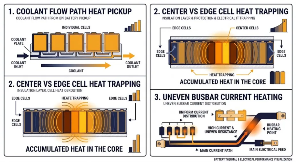
Temperature gradients rarely come from one single cause. Instead, three factors typically combine to create them.
Coolant Path Position
In a liquid-cooled rack, coolant usually enters at one point and exits at another, picking up heat along the way. Cells nearest the coolant inlet sit in cooler fluid. Cells nearest the outlet, by contrast, sit in fluid that has already absorbed heat from cells earlier in the path. As a result, outlet-side cells often run measurably warmer than inlet-side cells. This happens purely because of their position in the flow path, not because of anything different about the cells themselves.
Cell Position Within the Pack
Cells near the edge of a rack or enclosure sit closer to the outside walls, where some heat escapes to the surrounding air. Cells buried in the center of a dense pack, on the other hand, have neighbors on every side, so that heat has fewer places to go. Center cells, therefore, often run hotter than edge cells, even under identical cooling and identical current.
Current Path and Busbar Resistance
Current does not always split perfectly evenly across parallel cell groups. Small differences in busbar length, connection quality, or contact resistance mean some current paths carry slightly more current than others. Since heating from resistance follows I²R, even a small current imbalance produces a disproportionate heating difference. This connects directly to internal resistance variation covered in our cell matching guide: cells or groups with higher resistance generate more heat at the same current. As a result, a resistance mismatch and a temperature gradient often reinforce each other.
4. How a Temperature Gradient Accelerates Divergent Aging
Battery aging reactions speed up with heat. Researchers publishing in PMC (National Center for Biotechnology Information) found that inhomogeneous cell temperature inside a pack is a real, measurable driver of uneven degradation, not just a theoretical concern. Applied to a pack with a real gradient, this means the hottest cells are not just uncomfortable. They are quietly aging faster than their cooler neighbors, cycle after cycle.
This is where uneven heating and cell matching intersect. A pack that started out well matched, as covered in our cell matching guide, can still drift apart over time. A persistent hot zone can push those cells toward faster capacity fade. Meanwhile, cooler cells barely age at all. The BMS then has to work harder to compensate for a gap that thermal design, not manufacturing variance, actually created.
Cold cells create a different problem. Below their optimal range, cells deliver less power. They also accept slower charge rates. In practice, this means the coolest cells in a pack can become the limiting factor for dispatch power. This happens even though they are aging the slowest of anyone in the rack.
5. How the BMS Responds to What It Can Actually See
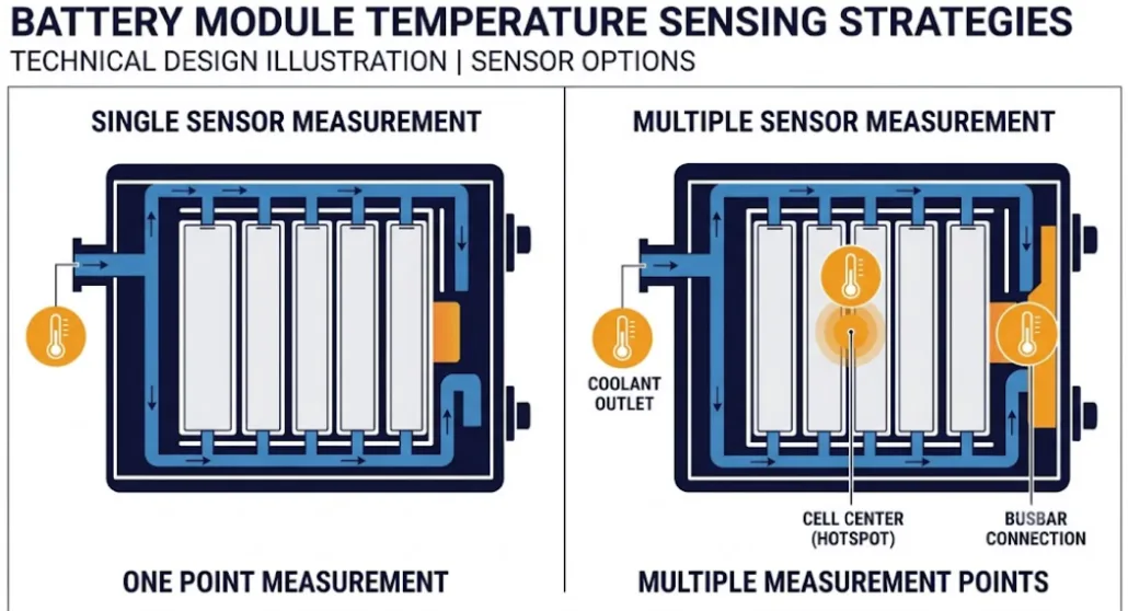
A BMS cannot manage a gradient it cannot measure. Sensor placement, therefore, matters as much as sensor accuracy. A design with one temperature sensor per module, placed at a single convenient point, will miss gradients happening between that sensor’s location and the rest of the module.
More thorough designs, instead, place multiple sensors per module. These sit at known high-risk points — near coolant outlets, at pack centers, and at busbar connections. This ties directly into the safety diagnostic algorithms covered in our BMS algorithms guide, since a BMS can only flag a developing hot spot if a sensor actually sits close enough to detect it before the gradient becomes a real problem.
6. Questions to Ask Your Supplier
What is your specified maximum cell-to-cell temperature gradient, not just the overall operating temperature range?
How many temperature sensors does each module have, and where are they physically placed?
For liquid-cooled systems, what is the coolant flow path? What gradient exists between inlet-side and outlet-side cells?
Do you have field or test data showing SOH divergence between hot-zone and cool-zone cells over time?
How does the BMS respond if a persistent gradient develops? Does it just log the data, or does it adjust balancing or dispatch limits?
Conclusion: A Temperature Gradient Is a Slow Problem That Looks Like No Problem at All
Overheating alarms are easy to notice. Temperature gradients, however, are not. A pack can run entirely within its safe range. It can still age unevenly, cell by cell. Nobody measured the gradient closely enough to see it. Ask suppliers for their specific gradient limit, not just their operating range. Then ask how many sensors actually watch for it.
For the manufacturing-stage half of this problem — how mismatched cells enter a pack in the first place — see our cell matching guide. Matching and thermal design solve two different sources of the same underlying issue: cells in one pack quietly drifting apart from each other over time.
☀️ Need a Thermal Design Review for Your BESS Project? Sunlith Energy reviews cooling architecture, sensor placement, and gradient specifications for BESS projects from 50 kWh upward. Contact us before you finalize a thermal design.
Frequently Asked Questions About Cell Temperature Gradients
What is a temperature gradient in a battery pack?
A temperature gradient is the difference between the hottest and coolest cell temperatures in a pack at the same moment, usually written as ΔT. It is a separate measurement from the pack’s overall operating temperature range. That is because a pack can sit within a safe range overall while still having a large gap between its warmest and coolest cells.
What causes temperature gradients inside a BESS pack?
Three factors typically combine to cause gradients. Coolant path position matters, since cells near a coolant outlet run warmer than cells near the inlet. Cell position within the pack matters too, since center cells trap more heat than edge cells. Finally, uneven current distribution from busbar resistance differences creates uneven I²R heating across parallel cell groups.
How does uneven heating affect cell aging?
Hotter cells within a gradient age faster than cooler cells in the same pack, since battery degradation reactions speed up with heat. Over time, this can widen the performance gap between cells, even in a pack that started out well matched. As a result, the BMS ends up compensating for a gap that thermal design created, rather than manufacturing variance.
What is a safe temperature gradient for a BESS pack?
Exact limits vary by manufacturer and system design. However, a maximum gradient of around 5°C is commonly specified for air-cooled and moderately cooled systems, while premium liquid-cooled systems often target 2-3°C. Always confirm the specific figure with your supplier rather than assuming a standard number applies.
How many temperature sensors does a BESS module need?
There is no single universal number. Still, a module with only one sensor at a single convenient location cannot detect a gradient occurring elsewhere in that module. More thorough designs, therefore, place multiple sensors at known high-risk points, such as near coolant outlets, pack centers, and busbar connections.
⚡ Quick Answer: What Is Cell Matching? Cell matching is the process of sorting battery cells by voltage, capacity, and internal resistance before they go into a pack, so cells with similar characteristics end up grouped together. It happens on the factory floor, before assembly. This is not the same thing as BMS balancing, which corrects drift after the pack is already built and in use. Skipping cell matching does not make a pack unsafe by itself, since the BMS still protects it. However, it does mean the BMS has to work much harder from day one. As a result, the pack’s real-world capacity and cycle life will likely fall short of what the cell datasheet promises.
1. Why Cell Matching Happens Before the BMS Gets Involved
Cell matching is a manufacturing step that happens before a single cell ever reaches a pack. Even cells from the same production batch are not identical. Small differences in electrode coating thickness, electrolyte fill, and formation cycling leave every cell slightly different. Capacity, voltage, and internal resistance all vary a little, even when the datasheet lists one number for all of them. In a single cell, this variation does not matter. Once dozens or hundreds of cells connect into a pack, though, it matters a great deal.
The BMS will eventually correct some of this drift through balancing, as covered in our complete battery management system guide. Cell matching, however, happens earlier. It is a manufacturing step, not a BMS function, and it exists to reduce how much correction the BMS has to do later.
2. Three Criteria Used to Sort Cells: Voltage, Capacity, and Resistance
Cell matching typically screens for three characteristics. Each one affects the pack differently. As a result, a thorough process checks all three rather than relying on just one.
Voltage (or SOC) matching — technicians group cells by their resting voltage after a defined charge or discharge point. This is the simplest check to run. It also catches the most obvious mismatches quickly.
Capacity matching — technicians charge and discharge test each cell to measure actual usable Ah, then group cells with similar capacity together. This matters most for series strings, since the lowest-capacity cell sets the ceiling for the whole string.
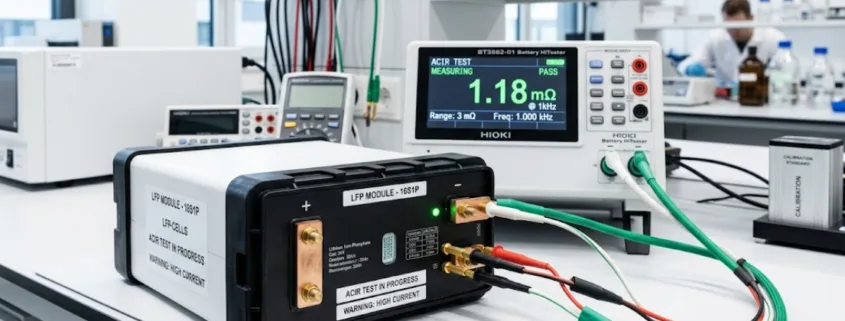
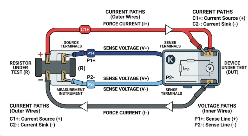
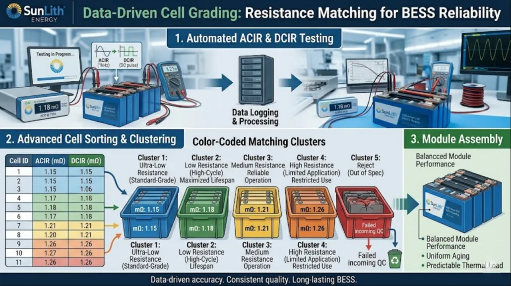
Internal resistance matching — technicians measure resistance using one of two methods, DCIR or ACIR, then group similar-resistance cells into the same parallel group. This matters most for parallel groups, since a lower-resistance cell otherwise takes more than its fair share of current.
High-volume manufacturers often combine all three, and internal resistance testing itself splits into two distinct methods worth understanding.
DCIR vs ACIR: Two Ways to Measure Internal Resistance
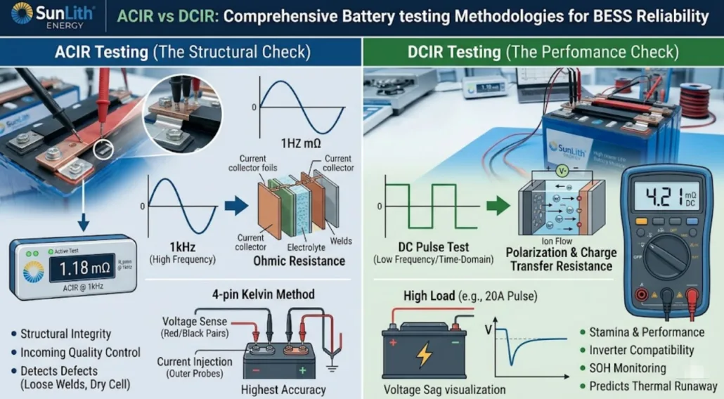
DCIR (DC internal resistance) testing applies a current pulse to the cell and measures the resulting voltage drop. Technicians then calculate resistance directly from Ohm’s law. This method closely reflects how the cell behaves under a real load, since it uses an actual current step rather than a small signal. The tradeoff is speed: each pulse needs time to apply and settle, which slows down high-volume sorting.
ACIR (AC internal resistance) testing instead applies a small alternating current signal, commonly at 1 kHz, and reads the resulting impedance directly. This method runs much faster than DCIR, which is why many production sorting lines use it as a first-pass screen. However, ACIR mostly captures the cell’s high-frequency ohmic resistance. It does not fully capture the slower electrochemical charge-transfer resistance that DCIR testing reveals.
In practice, many manufacturers use ACIR for fast first-pass screening across an entire incoming batch, then apply DCIR pulse testing to verify cells before they go into the same series string or parallel group. A supplier who only mentions one of these two methods is likely doing the faster, less thorough version alone.
3. Series Strings vs Parallel Groups: Different Priorities
Series and parallel connections fail differently when cells are mismatched. For this reason, they need different matching priorities.
In a series string, cells share the same current, but their voltages differ based on individual state. The weakest cell — the one with the lowest capacity — reaches its low-voltage cutoff first during discharge. Likewise, it hits its high-voltage cutoff first during charge. As a result, that one weak cell limits the usable capacity of the entire string. This happens even though the other cells still have energy left. This is why capacity matching matters most for series strings.
In a parallel group, cells share the same voltage, but current splits between them based on internal resistance. A cell with lower resistance pulls more current than its neighbors. In turn, it works harder and ages faster. Over time, that uneven current sharing can widen the resistance gap further, creating a feedback loop. Left unchecked, this loop drives localized accelerated aging in the same cells, cycle after cycle. That localized wear is what leads to premature pack failure, well before the rest of the pack reaches end of life. For a buyer, that translates directly into a shorter calendar life and a worse return than the datasheet cycle life implied. This is why resistance matching matters most for parallel groups.
☀️ Resistance matching matters most for parallel groups. 💡 The Thermal Feedback Loop: Internal resistance mismatch and localized heating reinforce one another. For a deeper look at how temperature imbalances accelerate this degradation, read our guide on Cell Temperature Gradients in BESS
4. What Happens If You Skip Cell Matching
Skipping cell matching does not make a pack dangerous on its own. A properly designed BMS still enforces voltage and temperature limits, regardless of how well matched the cells are. What changes, instead, is how hard the BMS has to work, and how much capacity the pack actually delivers.
If cells arrive at noticeably different SOC and go into a pack without matching, the BMS must run a large initial balancing pass. This happens the first time the pack charges. Passive balancing currents are typically small — often just tens to a few hundred milliamps — compared to the pack’s full Ah rating. Correcting a large initial mismatch this way can take many hours. In some cases, it takes several charge cycles before the pack reaches a properly balanced state.
Beyond the slow start, an unmatched pack often never fully closes the gap. If capacity variation between cells is large enough, ongoing balancing keeps the weakest cell from falling further behind. Still, balancing cannot manufacture capacity that a weak cell simply does not have. The pack’s usable capacity, therefore, ends up set by its weakest link, cycle after cycle.
5. Top-Balance vs Bottom-Balance: Which Comes First
When manufacturers match cells by connecting them in parallel before final assembly, the SOC point at which this happens changes the outcome.
Bottom-balance matching connects cells in parallel at a low SOC, often close to how they arrive from the manufacturer. This approach is simple and fast. However, it only aligns the cells at the bottom of the charge curve. The pack will likely still need a top-of-charge balancing pass once assembled and charged for the first time.
Top-balance matching, instead, charges the parallel-connected cells to a high SOC before final assembly, typically near the top of the charge curve. This produces a better-aligned pack from the first charge. That is because the region where mismatch matters most for safety and full capacity gets addressed early. The tradeoff is time: bringing a large batch of cells to a matched high-SOC state takes more equipment and more hours before assembly can begin.
6. Cell Matching at Scale: How Manufacturers Grade Cells for Utility BESS
At utility scale, matching thousands of cells by hand is not practical. Instead, high-volume manufacturers run automated sorting lines. These measure voltage, capacity, and resistance for every incoming cell. Grading software then groups cells into matched sets before they ever reach the assembly line.
For a BESS buyer, this raises a practical question worth asking directly: does the supplier grade and match cells before assembly, or does the pack rely entirely on the BMS to fix mismatch after the fact? Independent testing resources such as Battery University document just how differently DCIR and ACIR readings can diverge on the same cell, which is exactly why asking a supplier which method they use, and at which stage, is worth doing directly.
A supplier who can show incoming cell test data is doing meaningfully more quality control than one who simply points to their BMS’s balancing feature. Look, in particular, for a specific matching tolerance — for example, a defined percentage spread in capacity, or a defined milliohm band in resistance.
7. Questions to Ask Your Cell or Pack Supplier
Do you test and match cells by voltage, capacity, and internal resistance before assembly, or only one of these?
For internal resistance, do you use DCIR, ACIR, or both — and at which stage does each method apply?
What matching tolerance do you use? For example, what percentage spread in capacity, or what milliohm band in resistance?
Do you keep incoming cell test data on file? Can you provide it for the specific batch used in our order?
For series strings, how do you decide which cells go together — capacity, resistance, or both? Our BMS algorithms guide covers how the BMS itself later measures DCIR for SOH estimation, which is a useful comparison point when you ask this question.
Is matching done at a low SOC, a high SOC, or both, before final assembly?
Conclusion: Matching Sets the Ceiling the BMS Can’t Raise
A BMS is very good at correcting small, ongoing drift between cells. It is not designed, however, to compensate for a pack that started out badly mismatched. Cell matching before pack assembly sets the baseline the BMS then has to maintain for the life of the system. A well-matched pack lets the BMS do its normal job: fine-tuning small differences over time. A poorly matched pack, by contrast, forces the BMS into a losing battle against a gap it cannot close, cycle after cycle.
When evaluating a cell or pack supplier, ask specifically how they match cells before assembly, including whether they use DCIR, ACIR, or both. Do not just ask how the BMS balances them afterward. For supplier evaluation more broadly, see our BESS supplier BMS evaluation guide. The cell matching answer says a lot about how much real capacity and cycle life you can expect to see in practice.
☀️ Need Help Evaluating a Cell Matching Process? Sunlith Energy reviews incoming cell test data, matching tolerances, and pack assembly quality control for BESS projects from 50 kWh upward. Contact us before you finalize a cell or pack supplier.
Frequently Asked Questions About Cell Matching
Is cell matching the same as BMS balancing?
No. Cell matching happens before assembly. It is a manufacturing step that sorts cells by voltage, capacity, and internal resistance, so similar cells end up grouped together. BMS balancing, on the other hand, happens after assembly, correcting the small drift that develops during normal use. Matching reduces how much balancing the BMS has to do; it does not replace it.
What is the difference between DCIR and ACIR matching?
DCIR testing applies a current pulse and calculates resistance from the voltage drop using Ohm’s law, closely reflecting real load behavior. ACIR testing applies a small AC signal, commonly at 1 kHz, and reads impedance directly, which runs much faster but mostly captures high-frequency ohmic resistance rather than the full picture. Many manufacturers use ACIR for fast first-pass screening, then confirm with DCIR before final grouping.
What is the difference between capacity-based and resistance-based sorting?
Capacity-based sorting groups cells with similar usable Ah, and matters most for series strings, since the lowest-capacity cell sets the ceiling for the whole string. Resistance-based sorting, by contrast, groups cells with similar internal resistance, and matters most for parallel groups, since a lower-resistance cell will otherwise pull more than its fair share of current.
Does skipping this step make a battery pack unsafe?
Not directly. A properly designed BMS still enforces voltage and temperature limits, no matter how well the cells were matched. That said, skipping this step does mean the BMS must run a larger initial balancing pass. In turn, the pack’s real-world capacity may fall short of the datasheet value, since the weakest cell limits the whole pack.
Should I ask my BESS supplier for this test data?
Yes. Ask whether the supplier tests and matches cells by voltage, capacity, and internal resistance before assembly, and which resistance method they use. A supplier who can provide incoming cell test data for your specific batch is demonstrating a real quality control process, not just relying on the BMS to compensate after the fact.
Is top-balance or bottom-balance better?
Top-balance, which aligns cells at a high SOC before assembly, generally produces a better-aligned pack from the first charge. That is because it addresses the top-of-charge region where mismatch matters most. Bottom-balance is faster, but the pack will likely still need a top-of-charge balancing pass once assembled.
⚡ Quick Answer: What Is BMS Cycle Counting? BMS cycle counting turns raw current and SOC data into a wear metric. First, most systems track Ah/kWh throughput and convert it into Equivalent Full Cycles (EFC). Next, advanced platforms run a rainflow algorithm that splits a messy SOC trace into discrete, depth-weighted cycles. Finally, premium BMS platforms add a stress-weighted layer for C-rate and temperature. As a result, BMS cycle counting feeds SOH and RUL models, not just a simple warranty odometer.
BMS cycle counting sounds simple. In reality, it is one of the least understood functions inside a Battery Management System. Every BESS datasheet shows a number like “6,000 cycles to 80% SOH.” Few buyers ask the obvious follow-up question: how does the BMS actually reach that count in the field? A grid-connected battery rarely swings cleanly from 100% to 0% and back. Instead, it moves up 12%, down 4%, up 20%, down 7%, dozens of times a day. Dispatch signals, solar variability, and frequency-regulation events all drive this pattern. Because of this, converting a noisy trace into one clean cycle number is a genuinely hard firmware problem.
This guide explains exactly how BMS cycle counting works today. First, we cover why simple threshold counting fails for BESS. Next, we break down the rainflow algorithm, borrowed from mechanical fatigue analysis. Then, we show how it solves the partial-cycle problem. Finally, we explain why the datasheet number rarely matches what your BMS reports in the field. For the state-estimation layer this article builds on, see our guides to BMS SOC estimation methods and BMS algorithms explained.
1. Why BMS Cycle Counting Is Harder Than It Sounds
A cycle sounds easy to count: full charge, full discharge, done. However, “one cycle” has no single agreed definition outside the lab. A cell tested for its datasheet rating runs controlled, repeatable 100%–0% swings at a fixed C-rate and temperature. However, a cell inside a grid-connected BESS does nothing of the sort.
In practice, real-world SOC traces look like a jagged mountain range. Hundreds of small reversals happen every day. A dispatch instruction, a passing cloud, or a short frequency-regulation event can each trigger one. If BMS cycle counting logged every reversal as a cycle, one day of frequency regulation could register thousands of cycles. That would badly overstate wear. On the other hand, a threshold-only method misses just as much. A peak-shaving BESS that stays within the 20–80% band could show almost zero full cycles. Yet it may still have years of hard use behind it.
Neither outcome helps warranty tracking or SOH modelling. For this reason, BMS and EMS firmware rely on purpose-built cycle-counting algorithms instead of simple threshold logic. According to Energy-Storage.News, the industry still lacks one universal definition of a cycle. That gap is exactly why several competing counting methods exist side by side today.
The most basic form of BMS cycle counting sets two SOC thresholds, typically near 95% and 5%. Firmware then adds one to a counter each time the pack completes a full traverse between them. This approach is cheap to build and easy to explain. As a result, it shows up often in low-cost consumer BMS platforms.
For stationary BESS, though, this method falls short. Most BESS installations rarely complete a true top-to-bottom swing. Dispatch strategies deliberately avoid the SOC extremes to protect cycle life (see our guide on the 20/80 rule for batteries). Consequently, a system cycling between 20% and 80% SOC may never trigger a single “full cycle” under this method. That can happen even after years of heavy use. This undercount is precisely why the industry moved toward throughput-based BMS cycle counting instead.
3. Method 2: BMS Cycle Counting With Ah-Throughput (EFC)
This method sits behind almost every commercial BESS warranty. Rather than watching for full swings, the BMS integrates current over time. It uses the same Coulomb-counting math built for SOC estimation. In other words, it adds up every amp-hour that flows in or out of the pack, in either direction. The BMS then divides that cumulative throughput by the pack’s rated capacity. The result is Equivalent Full Cycles, or EFC.
For example, a 500 kWh BESS that has processed 1,000 kWh of cumulative throughput has logged 2 EFC. This version of BMS cycle counting is simple. In addition, it is cheap to run continuously. And it works no matter how the pack is actually cycled, since it never requires a full 100–0% swing.
The Core Blind Spot of EFC Tracking
EFC has one well-known limitation: it treats every amp-hour the same, no matter how deep the swing was. As Energy-Storage.News notes, EFC alone cannot tell one cycle at 100% depth of discharge apart from two cycles at 50% DoD, or ten cycles at 10% DoD. Yet these three patterns stress the cell chemistry quite differently. So, shallow frequent cycling and deep infrequent cycling can log an identical EFC number. Even so, they age the pack at very different rates.
Many BMS platforms partly correct for this. They re-base the EFC denominator against current estimated capacity instead of nameplate capacity. That keeps the figure accurate as the pack fades. Even so, the core blind spot remains. This gap is exactly what rainflow-based BMS cycle counting was built to close.
4. Method 3: Rainflow-Based BMS Cycle Counting for Partial Cycles
Rainflow counting began as a tool for mechanical fatigue analysis. Engineers used it to turn a noisy load history into a clean set of discrete stress cycles. Battery researchers later adapted the same logic for SOC traces. A peer-reviewed ScienceDirect study on grid-integrated BESS cycle counting confirms it as the most widely used cycle-counting algorithm in the field today. Rainflow-based BMS cycle counting solves what EFC cannot: it identifies the depth of every individual swing, not just the running total.
How the Rainflow Algorithm Works Step-by-Step
The BMS records every local extremum in the SOC trace. In other words, it logs every point where the pack switches from charging to discharging, or back again.
It then calculates the SOC delta between each set of three consecutive extrema.
Consequently, If the middle delta is smaller than or equal to both neighbours, that segment counts as one closed, complete cycle at that specific depth.
The BMS removes those two points. Then it repeats the comparison on the remaining trace — much like water draining off a stepped rooftop, which is where the algorithm gets its name.
The output is a list of discrete cycles, each tagged with its own depth of discharge. For example: “47 cycles at ~80% DoD, 1,200 cycles at ~15% DoD,” instead of one flattened EFC figure.
One detail matters here: rainflow-based BMS cycle counting applies to depth of discharge, not absolute SOC. A swing from 80% down to 70% and a swing from 20% down to 10% both register as the same 10%-DoD event. Both count as equivalent stress. This lines up with how degradation models actually work, since most treat wear as a function of cycle depth, not the absolute SOC band it happens in.
Because rainflow output preserves depth data, it feeds straight into the DoD-weighted models used by SOH and RUL algorithms. That is the same layer we cover in our guide to BMS algorithms explained.
5. Method 4: Stress-Weighted BMS Cycle Counting
The most advanced BMS and EMS platforms push rainflow-based BMS cycle counting one step further. Instead of tallying cycles by depth alone, each identified cycle passes through a stress function. That function also factors in the C-rate and cell temperature present during that specific cycle. For instance, a 60%-DoD cycle at 0.2C and 25°C is far gentler than the same 60%-DoD cycle at 1.5C and 40°C. A stress-weighted counter reflects that difference clearly.
Rather than reporting a raw cycle count, this method builds a running “degradation” or “aging” score. That score, not the raw EFC number, feeds the most accurate RUL models. This is also why two BESS units with an identical EFC count can end up with very different projected remaining life.
6. How Firmware Filters Noise Before BMS Cycle Counting Begins
Raw current-sensor data is noisy. Grid-frequency jitter, brief EMS corrections, and normal sensor tolerance all create tiny, meaningless direction reversals in the SOC trace. Sometimes there are hundreds per hour. Feed that data straight into a rainflow algorithm, and the result is an explosion of trivial micro-cycles. Those micro-cycles overstate wear.
To prevent this, production BMS cycle counting firmware applies a minimum-delta, or hysteresis, threshold. A direction reversal only counts as a genuine local extremum once SOC has moved by some minimum amount, commonly 1–2%. Only then does it enter the counting algorithm. Firmware treats smaller reversals as noise and ignores them.
This single design choice separates a BMS that produces warranty-defensible cycle data from one that does not. Set the threshold too low, and cycle counts inflate from sensor noise. Set it too high, and the BMS misses genuine shallow cycling that still adds to ageing. Therefore, always ask your BMS supplier what hysteresis threshold their firmware applies. Datasheets rarely publish this figure. Yet it directly shapes every downstream SOH and warranty number.
7. Comparing the Four Cycle-Tracking Methods
Method
What It Captures
DoD-Aware?
Best For
Main Limitation
Threshold counting
Full 95%–5% traverses only
No
Simple consumer packs
Badly undercounts partial-cycling BESS
Ah-throughput (EFC)
Cumulative current throughput
No
Warranty reporting, simple dispatch
Cannot distinguish deep vs. shallow cycling
Rainflow counting
Each discrete swing, by depth
Yes
SOH modelling, mixed dispatch profiles
More compute-intensive; needs clean extrema
Stress-weighted counting
Depth + C-rate + temperature
Yes
RUL prediction, warranty defensibility
Requires a validated stress model per cell type
Most premium BMS platforms do not rely on just one method. Instead, they report EFC for simple dashboards and warranty tracking. Meanwhile, they run rainflow and stress-weighted BMS cycle counting in the background to feed SOH and RUL models. If a supplier says their BMS “counts cycles” without naming a method, ask directly. The gap between threshold counting and stress-weighted rainflow counting can differ by an order of magnitude in reported wear.
8. Why Datasheet Numbers Rarely Match Real-World Wear
A supplier’s “6,000 cycles to 80% SOH” claim is almost always a lab-derived EFC figure. Labs measure it under fixed, controlled conditions. That means a specific depth of discharge, often 80–90%, a specific C-rate, often 0.5C–1C, and a specific ambient temperature, often 25°C. Change any one of these variables in the field, and the real cycle-life outcome shifts. Sometimes it shifts substantially. We cover this relationship in detail in our guide to how temperature affects LFP battery cycle life. You can also model your own scenario with our battery cycle life calculator. For a broader reference on stationary lithium battery testing conditions, see IEC’s battery safety and performance standards.
In practice, your BMS’s in-field EFC or rainflow-weighted count measures a different operating profile than the datasheet number. A BESS running frequent shallow cycles at moderate temperature may outlive its rated cycle count in calendar terms. Meanwhile, one running deep cycles at high ambient temperature may fall short of it. Neither outcome means the datasheet number was wrong. It simply means BMS cycle counting and lab-rated cycle life measure two related, but distinct, things.
9. Questions to Ask About Your Supplier’s BMS Cycle Counting Method
Which cycle-counting method does the firmware run: threshold, raw EFC, rainflow, or stress-weighted? A BMS that only reports raw EFC cannot show how deep-cycling patterns affect real degradation.
What minimum-delta, or hysteresis, threshold filters noise before a reversal counts as a cycle? An unpublished or unreasonably low threshold can quietly inflate cycle counts.
Is the EFC denominator based on nameplate capacity or current estimated capacity? Using nameplate capacity for the pack’s whole life understates EFC as the cell ages.
Does the cycle-counting output feed the SOH and RUL algorithms directly, or are they calculated separately? Disconnected pipelines often cause inconsistent SOH and warranty reporting.
What DoD, C-rate, and temperature conditions does the warranty’s rated cycle-life figure assume? This baseline is what your field cycle count should be compared against, not treated as a universal number.
Consider a 100 kWh BESS module running a frequency-regulation profile for one day. It discharges 8 kWh, charges 5 kWh, discharges 12 kWh, charges 10 kWh, discharges 6 kWh, and charges 9 kWh. That adds up to 50 kWh of cumulative throughput.
Decomposed into 3 discrete cycles at ~8%, ~12%, ~9% DoD
3 shallow cycles logged, none flattened into one number
While both numbers are technically correct, they answer different questions. The 0.50 EFC figure shows up on a simple throughput dashboard and feeds warranty-cycle tracking. The rainflow breakdown, however, is what a SOH model actually needs. Three shallow 8–12% DoD cycles age a cell differently than one 50%-DoD cycle would. That holds true even though both scenarios can produce the same EFC total.
Conclusion: BMS Cycle Counting Is a Modelling Choice, Not a Simple Tally
A BMS does not count cycles the way a person counts laps around a track. Instead, it reconstructs a cycle metric from a continuous current and SOC trace. Each method trades simplicity for accuracy differently. Threshold counting is too crude for real BESS dispatch. EFC is the industry-standard warranty metric, yet it stays blind to depth of discharge. Rainflow-based BMS cycle counting recovers that missing depth information. It breaks messy, real-world SOC traces into discrete, weighted cycles. Stress-weighted counting goes further still. It folds in C-rate and temperature to build the aging score that actually drives accurate RUL prediction.
For BESS buyers and operators, the lesson is simple. Do not take “the BMS tracks cycle count” at face value. Instead, ask which method it uses. Ask how it filters sensor noise. And ask how that number connects to the SOH and RUL figures you will eventually rely on for warranty claims and second-life valuation.
☀️ Need a BMS Cycle Counting and SOH Methodology Review? SunLith Energy reviews BMS cycle counting implementation, EFC and rainflow methodology, and SOH-RUL linkage for BESS projects from 50 kWh upward. Contact us before you commit to a supplier.
Frequently Asked Questions
How does BMS cycle counting work?
BMS cycle counting converts raw current and SOC data into a wear metric. Most systems first calculate cumulative Ah or kWh throughput. They then convert it into Equivalent Full Cycles. More advanced platforms add a rainflow algorithm on top. It breaks the SOC trace into discrete cycles at their true depth of discharge, filtering out small reversals below a set noise threshold.
What is an Equivalent Full Cycle (EFC) in BMS cycle counting?
An EFC is the standard unit behind most BMS cycle counting for warranty purposes. The BMS sums all Ah or kWh throughput — every unit of charge or discharge, in either direction. It then divides that total by the pack’s rated or current estimated capacity. Two cycles at 50% depth of discharge, and one cycle at 100% depth of discharge, both produce 1 EFC.
Why does depth of discharge matter if EFC already tracks total throughput?
Because EFC only tracks the total charge moved, not how it was distributed. A cell that goes through one deep 100%-DoD cycle experiences different stress than one that goes through ten shallow 10%-DoD cycles. Yet both can produce the same EFC total. Rainflow-based BMS cycle counting exists specifically to preserve this depth information for accurate SOH and RUL modelling.
What is rainflow counting, and why does BMS cycle counting use it?
Rainflow counting is an algorithm first built for mechanical fatigue analysis. Applied to a battery’s SOC trace, it identifies local turning points. It then pairs them into discrete, complete cycles at their true depth of discharge, instead of one flattened throughput number. This makes it the preferred method for BMS cycle counting on BESS platforms with irregular, partial-cycling dispatch profiles.
Why doesn’t my BESS ever seem to reach the cycle count on its datasheet?
The datasheet figure is almost always measured under fixed lab conditions: a specific depth of discharge, C-rate, and temperature. If your system cycles more shallowly, at a gentler C-rate, or at cooler temperatures, its real-world BMS cycle counting output accumulates more slowly than the lab figure implies. The reverse is true under harsher conditions.
Can two BESS units show the same cycle count but have different remaining life?
Yes. Raw EFC, and even simple cycle counts, do not capture the temperature and C-rate conditions each cycle occurred under. This is why advanced BMS cycle counting adds a stress-weighted layer. It produces a degradation score rather than a plain cycle number, which feeds more accurate Remaining Useful Life predictions than cycle count alone.
ACIR LFP battery testing is critical in Battery Energy Storage Systems (BESS). It checks each cell before assembly. As a result, it prevents hidden defects early.
In contrast, DCIR measures performance under load. However, ACIR focuses on physical structure. Therefore, it gives a fast and clear view of cell quality.
At SunLith Energy, every LFP cell is tested at 1kHz. Thus, only stable cells move forward.
The Science of ACIR LFP Battery Testing: Ohmic Resistance
ACIR uses a small alternating current to measure internal resistance. The signal runs at 1kHz.
Z=IV
Because the signal is fast, chemical reactions do not respond. Therefore, the result reflects only ohmic resistance.
What This Method Measures
Current collector resistance
Electrolyte conductivity
Weld integrity
Contact resistance
In short, it shows the physical build quality of the cell.
Why 1kHz is the Industry Standard for ACIR LFP Battery Testing
The 1kHz frequency is widely used. This is because it balances speed and accuracy.
At lower frequencies, chemical effects appear. On the other hand, very high frequencies add noise. Therefore, 1kHz gives stable readings.
As a result, this method provides:
Fast measurement
High repeatability
Clean data
High-Precision ACIR LFP Battery Testing via the Kelvin Method
Measuring milliohm resistance requires precision. Small cable resistance can affect results and lead to inaccurate data.
Therefore, engineers use the 4-pin Kelvin method.
How the Kelvin Method Works
Two probes inject current
Two probes measure voltage
Because of this separation, lead resistance is removed.
Key Benefits
Higher accuracy
Better consistency
True resistance values
Why ACIR Testing Improves BESS Reliability
Incoming Quality Control
First, this test detects defects early. For example, high resistance may indicate poor welds.
As a result, faulty cells are removed before assembly.
Cell Matching for Long Life
Next, uniform cells are critical. Otherwise, imbalance occurs.
If resistance varies:
Heat increases
Aging becomes uneven
Therefore, cells are grouped by similar values. This improves lifespan and stability.
Early Failure Detection
ACIR also helps detect early degradation.
For instance:
Rising resistance may signal internal damage
Sudden change may indicate failure risk
Thus, it supports predictive maintenance.
ACIR LFP Battery Testing vs DCIR
Both methods are important. However, they serve different roles.