Every BESS guide tells you to keep cells cool. Fewer explain why temperature has such an outsized effect in the first place. The Arrhenius relationship between temperature and battery degradation answers that question. It is not a rule of thumb. Instead, it is real chemistry. Understanding it changes how you think about thermal design.
This guide skips the practical checklist most temperature guides repeat. It explains the actual mechanism instead. First, it covers what the Arrhenius equation says. Then it covers why that equation applies to batteries at all. Then it covers a detail most guides skip. Cold accelerates aging too, through a completely different pathway than heat. Finally, it covers what this means for BESS design at scale.
Quick Answer The Arrhenius relationship between temperature and battery degradation describes how chemical reaction rates, including the ones that degrade a battery, scale exponentially with temperature. As a rough rule, degradation reactions roughly double in rate for every 10°C increase. This is not linear. A cell running 20°C hotter than another does not age twice as fast. It can age four times as fast or more.
Temperature Battery Degradation Arrhenius: What the Equation Actually Says
Chemistry students learn the Arrhenius equation for a reason. It shows up almost everywhere reaction rates matter. Battery degradation is, at its core, a reaction rate problem.
The equation behind the Arrhenius relationship between temperature and battery degradation is simple in shape. It links reaction rate to temperature through one key number: activation energy. Every chemical reaction needs a minimum amount of energy to proceed. This includes the side reactions that consume lithium inside a cell. Temperature sets how many molecules have enough energy to clear that bar at any given moment. Raise the temperature, and more molecules clear it. The reaction speeds up. It speeds up exponentially, not in a straight line.
This is why a common shorthand holds up well across a useful range. Degradation roughly doubles for every 10°C rise. It is a simplification of the real curve. Still, it captures the core idea. Small temperature increases produce big jumps in degradation rate.
Why Activation Energy Varies by Material
First, not every part of a battery responds to temperature the same way. Activation energy is specific to each material and each reaction. That number determines how sensitive a given process is to heat.
Research measuring activation energy across battery materials found real differences. This number is a key input for modeling the Arrhenius relationship between temperature and battery degradation. Graphite, the typical anode material, showed a low activation energy of about 0.025 eV. LFP, by contrast, showed a notably higher activation energy of about 0.116 eV. A higher activation energy generally means a steeper response to temperature changes. That shows up in how the material conducts and how it ages. Worth noting: this figure comes from a battery-testing equipment vendor’s own case study, not a peer-reviewed paper. The methodology is transparent and the number checks out, but it sits in a different sourcing tier than a journal citation.
This matters for a simple reason when applying the Arrhenius relationship between temperature and battery degradation to a real system. Generic degradation guidance often gets built around chemistries like NMC, not LFP specifically. Borrowing that number for an LFP system can produce a genuinely wrong degradation estimate. Accurate modeling needs an activation energy number that matches the real chemistry in the cell.
Temperature Battery Degradation Arrhenius: Why Cold Also Accelerates Aging
Most practical guides frame temperature as a single dial. Hotter is worse, colder is better, full stop. But the real picture is more interesting than that. It matters for how you design a system.
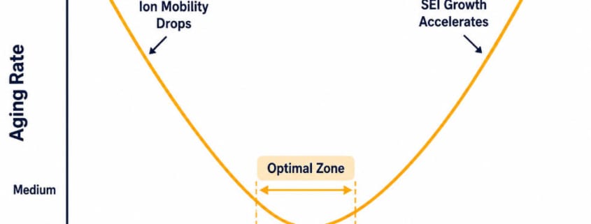
Research plotting battery aging rate against temperature found something specific. That research plotted the Arrhenius relationship between temperature and battery degradation directly. It is a V-shaped curve. Aging rate is not lowest at the coldest temperature tested. Instead, it hits a minimum at some optimal middle temperature. Then it rises again as conditions get colder still. Both ends of the curve show accelerated aging. Only the mechanism differs. Worth noting: the underlying study used NCA and NMC111 cells, not LFP. The V-shape itself is generally treated as chemistry-general in the literature, but the exact crossover point likely shifts somewhat for LFP specifically.
First, on the hot side, the story is the one covered above. Heat speeds up SEI growth and other side reactions directly. This runs through the same Arrhenius relationship covered above. For the deeper chemistry behind that specific mechanism, see our guide on SEI Layer Growth and Lithium Plating in LFP Cells. It covers the heat-driven side in full.
Then on the cold side, the mechanism is different. First, ion mobility slows down. Then internal resistance rises. Under high current in the cold, this can push cells toward lithium plating conditions. That is a different, worse outcome than simple slow aging. Instead, the V-shape is not really one curve. Instead, it is two separate degradation pathways overlapping. One dominates at high temperature. The other dominates at low temperature. A sweet spot sits in between, where both are minimized.
Temperature Battery Degradation Arrhenius and the Calendar vs Cycle Aging Link
Temperature does not degrade a battery through one single pathway. Instead, it touches both of the two aging processes that run in every cell at once.
Calendar aging is the slow degradation that happens even at rest. It follows the Arrhenius relationship closely. A cell sitting idle in a hot enclosure loses capacity faster than an identical cell sitting idle in a cool one. That difference comes purely from elevated reaction rates. Cycle aging is the degradation from active charging and discharging. It gets a second temperature effect layered on top. Heat during active cycling adds mechanical and chemical stress. This goes beyond what calendar aging alone would predict.
For the full breakdown of how these two aging pathways interact, see our guide on Calendar Aging vs Cycle Aging in LFP Batteries. It covers how operators separate them in real data. Temperature is the variable that connects both halves of that picture.
Applying This at BESS Scale: Why Uniformity Matters as Much as Average Temperature
Individual cell chemistry is only half the story. A BESS is not one cell. Instead, it is thousands of cells. The Arrhenius relationship has a brutal implication for how they age together.
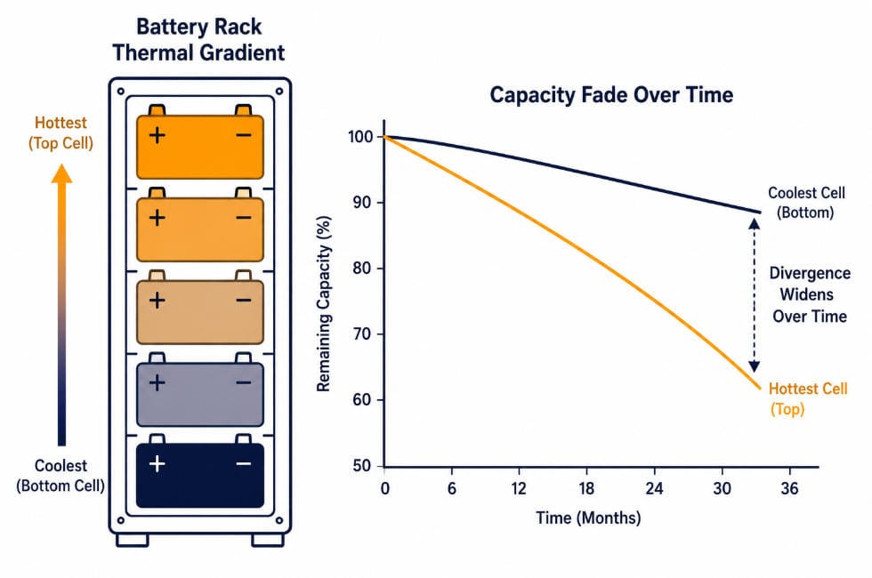
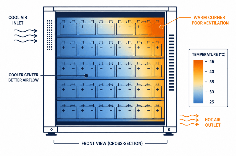
Degradation rate scales exponentially with temperature, not in a straight line. Small temperature differences between cells in the same rack do not average out. Instead, they compound. A cell running just a few degrees hotter than its neighbors ages meaningfully faster on its own. This can come from airflow patterns or its position in the rack. Over years of operation, that early divergence widens rather than closing. The hotter cell keeps aging faster at every step.
This is exactly why temperature uniformity across a BESS matters as much as the average temperature target. For the detailed engineering breakdown of safe temperature spread limits, see our guide on Cell Temperature Gradients in BESS. It covers what causes uneven heating in a rack. The Arrhenius relationship explained here is the underlying reason that guide’s ΔT limits exist in the first place.
Putting a Number on It: A Simple Arrhenius Comparison
The exponential relationship is easier to trust with a concrete example. Take two identical LFP cells. One runs at a steady 25°C. The other runs at 45°C, a 20°C difference that is common between a well-cooled and a poorly-cooled enclosure.
Using the 10°C-doubling shorthand, the hotter cell does not age 20% faster or even 50% faster. It ages roughly four times faster, since two separate 10°C jumps each roughly double the rate. A design choice that looks like a modest thermal compromise on paper can matter a lot in practice. It can translate into a dramatically shorter real-world service life. This is the practical payoff of understanding the Arrhenius relationship instead of just following a cooling checklist blindly.
The same logic applies in reverse. Pulling a system from 45°C down to 35°C can meaningfully extend service life. That is still a fairly warm operating point. It still runs warmer than the 25°C reference point most datasheets use. Incremental cooling improvements pay off at every point along the curve, not just at the extremes.
What This Means for Thermal Design Choices
None of this changes the practical playbook much. Still, it explains why that playbook works the way it does.
Liquid cooling outperforms air cooling on more than comfort. It holds cells within a tighter temperature band. It also reduces cell-to-cell spread. Both matter directly because of the exponential relationship covered above. For the full comparison of cooling approaches, see our guide on Liquid vs Air Cooling System Use in BESS. It covers the tradeoffs in detail. Cold-climate design deserves the same weight as hot-climate design, not less. The V-shaped curve means both extremes carry real degradation risk. For that side of the picture, see our guide on Cold-Climate BESS Design. It covers discharge-side cutoffs in cold weather.
For a practical, rule-of-thumb breakdown of temperature’s effect on cycle life, see our existing guide on Impact of Temperature on LiFePO₄ Batteries Cycle Life. It applies the 10°C-doubling shorthand to real cycle numbers. That guide covers the practical numbers. This one covers the mechanism behind them.
Temperature Battery Degradation Arrhenius: Quick Reference
Factor
What It Means
Core relationship
Degradation rate scales exponentially with temperature, not linearly
Common shorthand
Roughly doubles per 10°C temperature increase
Activation energy
Chemistry-specific; higher values mean steeper temperature sensitivity
Hot-side mechanism
Accelerated SEI growth and side reactions
Cold-side mechanism
Slower ion mobility, higher resistance, elevated plating risk under load
Curve shape
V-shaped, with a minimum-aging point, not a straight line
BESS-scale implication
Uniformity matters as much as average temperature, due to compounding
Frequently Asked Questions
In the Arrhenius relationship between temperature and battery degradation, does the 10°C-doubling rule apply exactly, or is it a simplification?
It is a simplification. The real relationship is a smooth exponential curve. The doubling shorthand holds up reasonably well across a normal operating range. Still, it is an approximation, not an exact law.
Why does LFP have a different activation energy than other chemistries?
Activation energy depends on the specific materials and reactions involved. LFP’s cathode chemistry behaves differently from NMC or NCA under the same conditions. Its measured activation energy differs as a result. Generic lithium-ion guidance does not always transfer cleanly as a result.
Is cold temperature ever actually good for battery life?
There is a minimum-aging point, and it sits below room temperature for some cells. But going too cold introduces its own accelerated aging pathway. Slower ion mobility and higher plating risk drive it. Colder is not simply better without limit.
Under the Arrhenius relationship between temperature and battery degradation, does uniformity really matter more than average temperature?
Both matter, but uniformity is the more commonly underestimated factor. Degradation compounds exponentially. A hotter pocket of cells in an otherwise well-managed system can become a persistent weak point. Over time, that weak point drags down pack-level performance.
Most cold-weather BESS design attention goes to charging. Lithium plating below roughly 0°C is a real, well-documented risk. Charge-inhibit logic is standard practice for good reason. Discharge-side cold behavior gets far less coverage. But it drives a different problem: resistance-driven voltage sag that trips a cutoff long before the pack is actually empty. This guide covers cold-climate BESS design for the discharge side specifically. It covers how cold amplifies the same DCIR mechanism covered in our dynamic cutoff design guide. It also covers what that means for current de-rating, heater sizing, and enclosure insulation.
⚡ Quick Answer Cold-climate BESS design has to account for LFP internal resistance rising sharply as temperature drops, since ion mobility slows in the electrolyte and at the electrode interface. This increases voltage sag under load, which can trip a fixed or even a DCIR-adaptive cutoff early if the resistance lookup table doesn’t extend to true cold-climate minimums. The design response has three parts: extending the cutoff’s temperature matrix to cover real winter conditions, applying current de-rating as temperature drops, and sizing enclosure heating and insulation to keep cells out of the steepest part of the resistance curve.
Why Cold-Climate BESS Design Needs to Address Discharge-Side DCIR
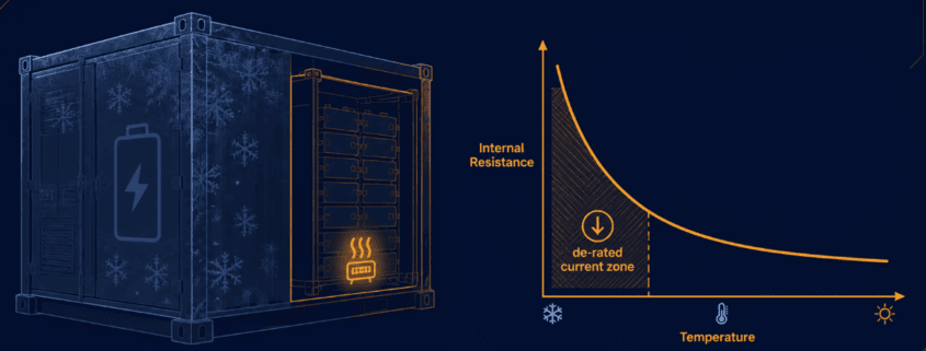
Our DCIR-adaptive cutoff design guide covers how internal resistance rises with cell age. It also covers how a fixed cutoff voltage fails to account for that rise. Cold temperature drives the same mechanism through a different cause. As temperature drops, electrolyte viscosity increases and ionic mobility slows, both in the bulk electrolyte and at the electrode interface. That raises internal resistance independent of cell age or cycle count. A fresh cell at -10°C can show meaningfully higher resistance than an aged cell at 25°C.
The practical effect is the same voltage-sag mechanism covered in the cutoff design guide.
Vterminal = VOCV − I × DCIR
A higher DCIR term means more sag at identical current, which reaches a fixed trip voltage sooner. This isn’t a marginal effect. A coupled electrochemical-thermal model validated against real cells from -20°C to 45°C confirms resistance rises sharply as temperature drops. Usable discharge capacity falls well below nameplate rating in the -10°C to -20°C range. That drop is driven primarily by the resistance rise, not by any real loss of stored charge. The energy is still in the cell. The pack just can’t deliver it fast enough to clear the cutoff threshold at typical discharge rates.
This matters most for anyone who has already implemented a DCIR-adaptive cutoff per our earlier guide. Say the HPPC test matrix behind that lookup table stopped at a moderate low-temperature bound, rather than the site’s true winter minimum. In that case, the adaptive cutoff extrapolates poorly. It can even fail safe into overly conservative behavior — exactly in the conditions where it matters most.
Extending the Cutoff Matrix for Cold-Climate BESS Design
The fix is directly upstream of implementation, not a separate system. The HPPC test campaign behind a DCIR-adaptive cutoff needs a temperature range that matches real deployment conditions. It shouldn’t just reflect a generic qualification range. A system specified for a temperate climate, but deployed somewhere with regular sub-zero winter lows, needs its lookup table re-tested. It needs to be rebuilt for that colder range. That should happen before commissioning, not patched in after a field failure.
Two practical points from that testing process carry directly into cold-climate design:
Pulse-test resistance at temperature steps that bracket the real minimum with margin, not just the design spec’s stated floor. Local weather can exceed nameplate assumptions during extreme events.
Re-validate hysteresis settings at cold temperature specifically. A cutoff tuned for hysteresis behavior at room temperature can behave differently at the steeper part of the resistance curve. There, small current fluctuations produce larger voltage swings.
Current De-Rating Strategy for Cold-Climate BESS Design
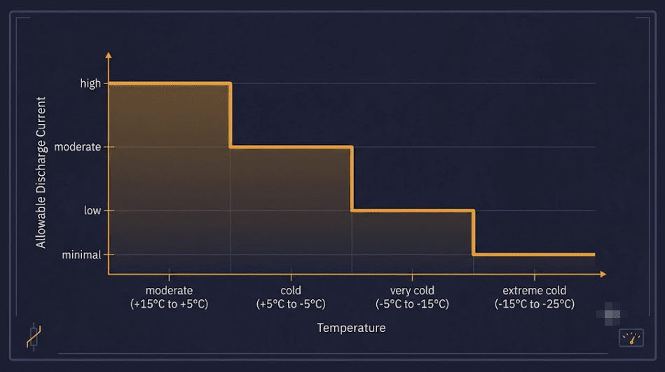
Even with an accurate cold-temperature resistance map, discharging at full rated current in cold conditions is risky. It pushes the system into the steepest part of the resistance curve. That’s where voltage sag grows fastest per unit of additional current. Current de-rating reduces the maximum allowed discharge current as measured cell temperature falls. It keeps the operating point away from that steep region. That’s safer than relying on cutoff logic alone to catch the problem after the fact.
A practical de-rating curve ties allowable current to the same temperature bands used in the DCIR lookup table. It steps down current limits at each band, rather than applying one blanket reduction across the entire cold range. This preserves as much usable power as safely possible at moderately cool temperatures. It pulls back harder as conditions approach the pack’s true low-temperature floor.
Heater Sizing for Enclosure Thermal Management
Where current de-rating manages the symptom, enclosure heating addresses the cause. It keeps cells out of the steep-resistance temperature range in the first place. A Sandia-led modeling study across eight U.S. locations found that enclosure heating and cooling loads alone increased required battery energy capacity. The increase ranged from 42% to 300%, depending on climate severity. The same study found that power conversion system placement matters too. Keeping the PCS inside the thermally managed envelope reduced the capacity penalty; leaving it exposed outside increased it. That model was built around an NMC cell, not LFP. LFP chemistry is generally more resistance-sensitive in cold conditions. So the real capacity penalty for an LFP system is likely at or above this range, not below it.
Heater sizing follows standard enclosure thermal design practice. Calculate steady-state heat loss for the enclosure’s surface area and target ΔT. Then apply a safety margin, commonly in the 125–130% range. That covers thermal mass and startup transients, not just steady-state loss. Insulation quality changes this calculation substantially. A well-insulated enclosure can cut steady-state heat loss by roughly 90% compared to an equivalent bare-metal enclosure. That’s normally the larger lever before reaching for a bigger heater.
Insulation and Enclosure Strategy in Cold-Climate BESS Design
BESS enclosures almost always use sealed-loop climate control rather than direct outside-air ventilation. Pulling ambient air through the battery compartment introduces humidity, salt, and dust. Those contaminants degrade cells and can create insulation-resistance faults over time. A cold-climate site often adds condensation risk too, from indoor-outdoor temperature swings. The standard architectures are a split air-conditioning unit with a sealed evaporator inside the compartment, for small to mid-size systems. Larger systems, above roughly 1 MWh or with high C-rate demands, typically use liquid cooling with cold plates instead. Whichever architecture is used, insulation determines how hard the heater has to work. It’s what holds the compartment above the steep-resistance zone, making it a critical factor in overall cold-climate BESS design. That’s worth specifying to the actual climate data for the site, not a generic regional assumption.
Bringing It Back to the Cutoff and Estimation Layers
Cold-climate design doesn’t introduce a new subsystem. It extends the temperature range that two subsystems already covered in this series need to handle correctly. The DCIR-adaptive cutoff’s lookup table needs a temperature axis that reaches the site’s true minimum. An EKF-based SOC estimator built from the same HPPC campaign needs its equivalent circuit model fitted across that same cold-temperature range. A model that only saw moderate temperatures during characterization will estimate poorly outside that range. Our EKF SOC estimation design guide and DCIR-adaptive cutoff design guide both assume the underlying test matrix covers real operating conditions. Cold-climate deployment is where that assumption needs the most scrutiny.
Key Takeaways
Cold-climate BESS design starts with the same electrolyte-viscosity and ion-mobility mechanisms that raise LFP internal resistance with age. That resistance rise produces the same voltage-sag effect that drives premature cutoffs. A DCIR-adaptive cutoff only protects against this if its HPPC test matrix extends to the site’s real winter minimum. A generic qualification range isn’t enough. Current de-rating tied to temperature bands keeps the operating point out of the steepest part of the resistance curve. That’s safer than relying on cutoff logic alone. Enclosure heater sizing should follow standard steady-state-plus-safety-margin methodology, with insulation quality as the larger lever before increasing heater capacity. Cold-climate design extends the same estimation and cutoff systems covered elsewhere in this series, rather than requiring a separate architecture.
Frequently Asked Questions
Does a DCIR-adaptive cutoff automatically handle cold-climate conditions?
Only if the HPPC test matrix used to build its lookup table extends to the site’s real winter minimum temperature. A table built against a generic or moderate qualification range will extrapolate poorly at true cold-climate lows. That can produce either an unsafe cutoff or an overly conservative one.
Is current de-rating necessary if the enclosure is heated?
Even a well-heated enclosure has a startup period. It can also see localized cold spots before reaching steady state. Current de-rating remains a useful safeguard during that transition. It’s not made redundant by heating alone.
How much does insulation actually reduce heater size?
A well-insulated enclosure can cut steady-state heat loss by roughly 90% compared to an equivalent bare-metal enclosure. That’s typically a larger lever than increasing heater wattage on a poorly insulated design.
Three failure modes show up again and again in LFP BESS operation. SOC readings drift from reality. Cells pull apart from each other in service. Cutoffs trip before the pack is actually empty. Most teams treat SOC drift and cell imbalance and premature cutoffs as three separate bugs. They are not. All three trace back to one root cause: LFP’s flat voltage curve. This guide covers SOC drift and cell imbalance and premature cutoffs as one connected design problem, not three separate ones, and shows where to fix each layer.
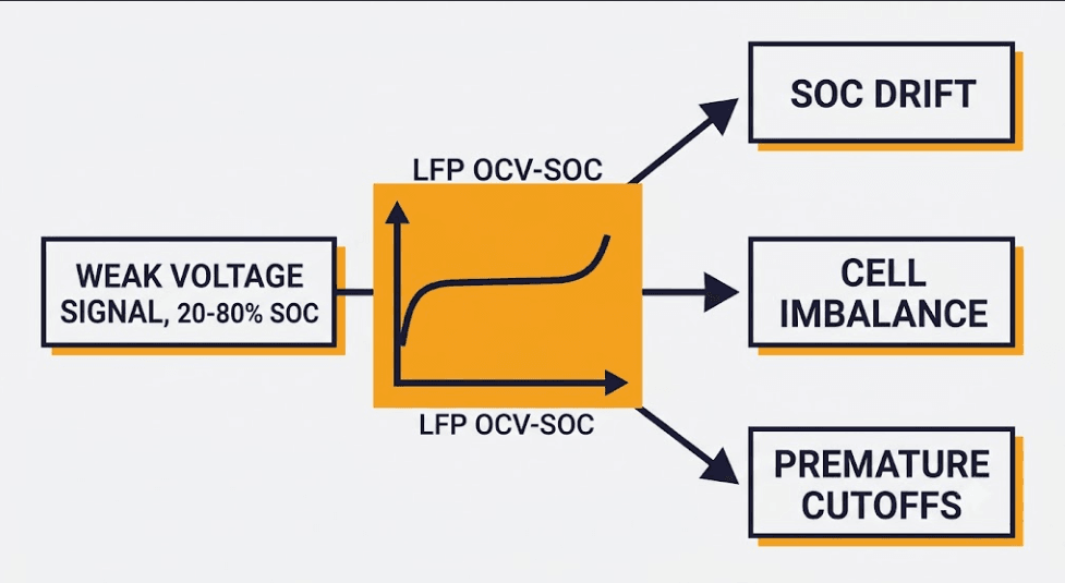
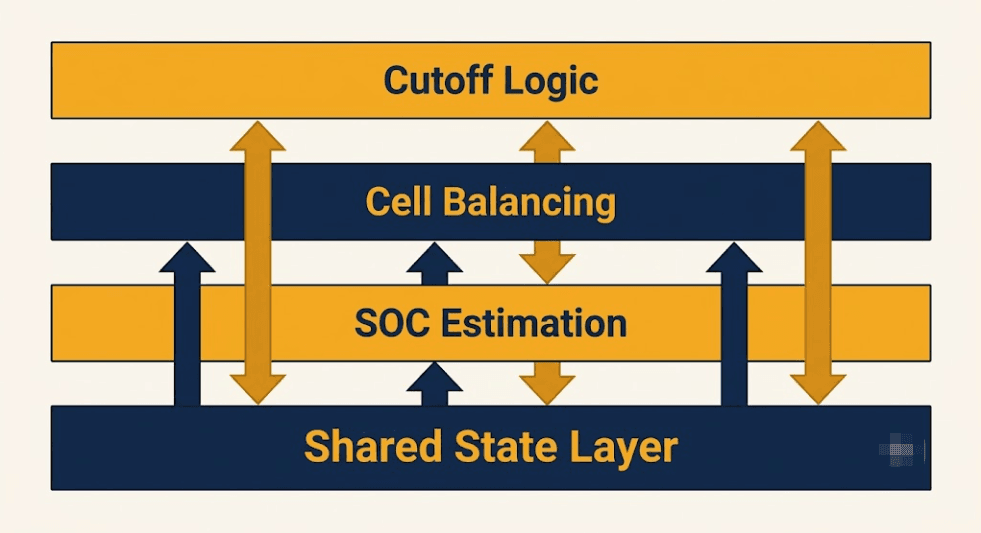
⚡ Quick Answer SOC drift and cell imbalance and premature cutoffs in an LFP BESS all stem from the same root cause. LFP’s flat OCV-SOC curve gives weak voltage signal across most of the operating range. Fixing this needs a matched design at three layers: SOC estimation (the model), cell balancing (the pack), and cutoff logic (the trip point). All three should share one live state, instead of running as separate modules.
Why LFP’s Flat Voltage Curve Drives SOC Drift and Cell Imbalance
LFP cells sit near 3.2–3.3V across roughly 80% of their usable range. A cell at 30% SOC looks almost identical to a cell at 70% SOC on voltage alone. This flat region is the reason SOC drift and cell imbalance and premature cutoffs all show up together in the same systems.
Weak voltage signal means SOC estimation has little to correct against. As a result, it drifts unless the model is built carefully. Weak voltage signal also means cell-to-cell differences hide longer before anyone notices. A pack can drift out of balance for weeks before the voltage spread becomes visible. Furthermore, a weak voltage signal means a cutoff tuned only to a fixed trip voltage cannot tell resistance-driven sag from real depletion. It trips early, stranding capacity the cell still has.
None of these three problems is really about SOC, balancing, or cutoffs on their own. SOC drift and cell imbalance and premature cutoffs are all downstream of the same flat curve. That is why fixing them one at a time, in isolation, tends to under-deliver.
Designing the SOC Estimation Layer for SOC Drift and Cell Imbalance
The estimation layer needs a model, not just a lookup table. LFP’s flat curve makes simple OCV lookup unreliable during operation. Coulomb counting works but drifts without a reset point, and that drift compounds with cycling. An Extended Kalman Filter, built from an equivalent circuit model fitted to HPPC test data, corrects itself continuously against tiny voltage signals that other methods miss.
Getting this layer right matters beyond the SOC number itself. A biased estimate feeds false signals into the other two layers, discussed below. Our EKF SOC estimation design guide covers the model-building and covariance-tuning steps in full.
Mitigating In-Service Cell Imbalance and SOC Drift
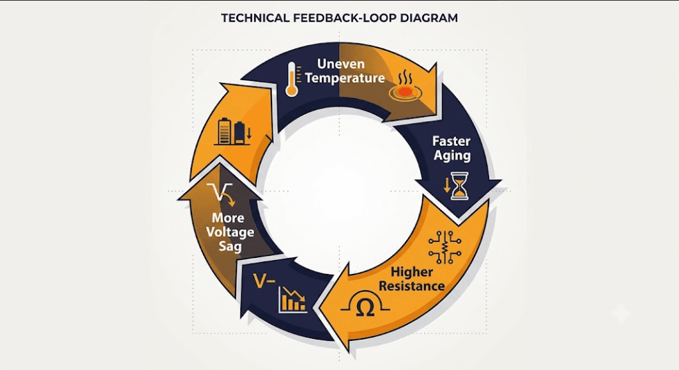
Cell imbalance is not just a factory-matching problem. Even a well-matched pack drifts apart over years, driven mainly by uneven heat. A cell running a few degrees hotter ages faster, gains resistance faster, and sags more under load — which can push it hotter still. Left unmanaged, that feedback loop turns a small temperature gap into a real capacity gap.
Design against this at two levels: thermal layout, sized around worst-case gradients rather than pack averages, and balancing topology matched to the cycling profile. Light daily cycling tolerates passive balancing. Heavy cycling or a persistent thermal gradient needs active balancing to keep pace. Our in-service cell imbalance guide covers both levers in depth.
Designing a Dynamic, DCIR-Adaptive Cutoff
A fixed cutoff voltage assumes fresh-cell resistance at room temperature. Real packs age and get cold. Their internal resistance rises on both counts, sagging more under identical load, which trips a static cutoff earlier and earlier even though real capacity remains.
A DCIR-adaptive cutoff fixes this by calculating the trip voltage in real time. It uses measured current and a resistance value pulled from an HPPC-derived lookup table, indexed by SOC, temperature, and cell age. This alone recovers up to 10% of effective throughput in mid-to-late project life that a static cutoff would otherwise strand. Our DCIR-adaptive cutoff design guide covers the full lookup-table structure.
Closing the Loop: Sharing State Across All Three
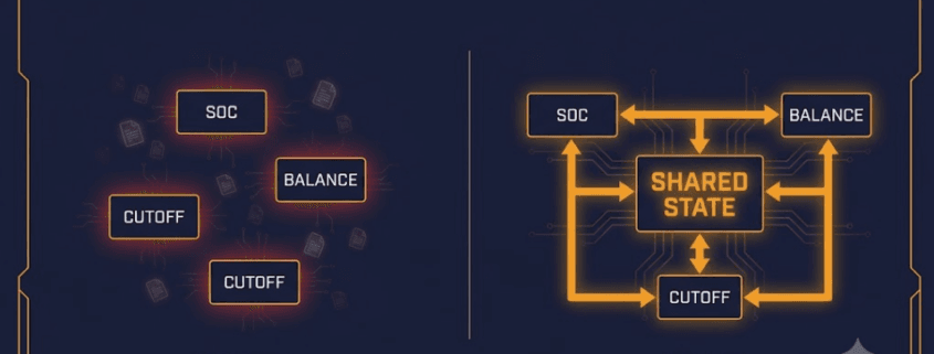
Building these three layers correctly in isolation still leaves a gap. This is where SOC drift and cell imbalance and premature cutoffs stop being separate design problems and start needing one shared answer. Each layer can run its own internal estimate of pack state, and small timing differences let those estimates quietly disagree. The estimator’s SOC value, the balancer’s voltage-spread reading, and the cutoff logic’s resistance calculation should all reference the same live data, not three separate copies of it.
This shared-state design also creates a natural place to catch developing faults. A cell whose resistance departs sharply from its neighbors is worth flagging. This matters most when that departure doesn’t track the pack’s overall aging trend. It’s a signal that’s much harder to catch when each subsystem only sees its own narrow slice of the picture. Our integrated BMS control architecture guide covers how to build that shared layer without a full BMS redesign.
How This Differs From a Buyer’s Checklist
This guide is a design reference, not a procurement checklist. If you’re evaluating a supplier’s BMS rather than architecting one, our BMS for LiFePO4 batteries guide covers the specs and questions to ask before you buy. If your problem sits further upstream — sorting and matching cells before a pack is even assembled — see our cell matching before pack assembly guide. This guide picks up once the pack is designed and in service, addressing SOC drift and cell imbalance and premature cutoffs as they actually show up over years of operation.
This same coordination challenge shows up in the research too. A study on distributed Kalman filtering across battery pack cells explores this tradeoff for thermal estimation specifically, finding that distributed approaches can track a centralized estimate closely when properly designed — the same coordination problem this guide addresses for SOC, balancing, and cutoff logic. Get that coordination wrong, and the failure mode this guide’s shared-state approach is built to avoid shows up instead.
Key Takeaways
SOC drift and cell imbalance and premature cutoffs are not three unrelated bugs — they are one shared-root-cause design problem. All three trace back to LFP’s flat OCV-SOC curve, which gives weak voltage signal across most of the operating range. Fix the estimation layer with a properly parameterized and tuned EKF, not a raw lookup table. Imbalance gets fixed at the thermal-layout and balancing-topology level, not just at factory cell matching. Cutoffs need a DCIR-adaptive design that accounts for real-world resistance, not a fixed datasheet value. Then close the loop: share state across all three layers so they reinforce each other instead of quietly disagreeing.
Frequently Asked Questions
Are SOC drift, cell imbalance, and premature cutoffs really connected problems?
Yes. All three trace back to LFP’s flat voltage curve, between roughly 20% and 80% SOC. That curve gives weak signal for SOC estimation. It hides cell-to-cell differences longer. It keeps a fixed cutoff from telling resistance sag apart from real depletion.
Do I need to fix all three layers at once?
Not necessarily in one project phase, but design them with the same shared-state architecture in mind from the start. Retrofitting shared state after each layer was built in isolation is more work than designing it in from the beginning.
How is this different from a standard BMS buyer’s guide?
A buyer’s guide covers what specs and questions to check before purchasing a BMS. This guide covers how to design or tune those systems once you own the architecture — the estimation model, the balancing strategy, and the cutoff logic itself.
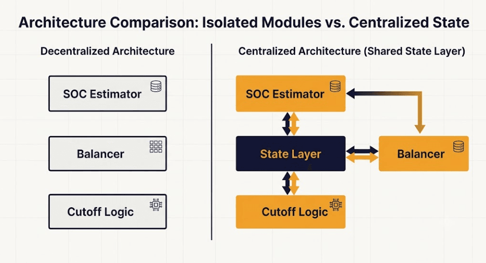
Most BMS designs treat SOC estimation, cell balancing, and cutoff protection as three separate modules. Each one runs its own logic. Each one reads its own inputs. This works, but it leaves value on the table. An integrated BMS control architecture ties these three functions together instead. They share one live state, not three separate guesses. This guide covers what that shared state looks like, and why it matters for LFP. New to BMS fundamentals first? Our BMS explained guide covers the basics before returning here.
⚡ Quick Answer An integrated BMS control architecture means the SOC estimator, the cell balancer, and the cutoff logic all read from one shared, current view of each cell’s voltage, resistance, and temperature. Without this link, each subsystem can act on a slightly different picture of the pack, and small disagreements between them compound into real errors.
Why Three Separate Modules Create Hidden Errors
This challenge is related to a broader question in battery-pack monitoring: whether separately-run, local estimators can be trusted to agree with a fully centralized view. Research on distributed Kalman filtering across battery pack cells explores this tradeoff for thermal estimation specifically, finding that distributed approaches can track a centralized estimate closely when properly designed — the same coordination problem this article addresses for SOC, balancing, and cutoff logic. A BMS built as three separate modules seems simpler at first. But each module often keeps its own internal estimate of pack state. The estimator has its own SOC value. The balancer has its own view of cell voltage spread. The cutoff logic has its own read on present resistance. These three views should agree. In practice, small timing gaps and separate filtering choices let them drift apart, even by a small amount.
A Concrete Example of the Problem
Picture a cell under a sudden high-current pulse. The estimator’s filter may lag the true voltage sag. The lag can run a few hundred milliseconds. The cutoff logic reads raw current and voltage directly. So it reacts faster. It might trip a cutoff. The estimator’s own SOC value says this should not happen yet. Without shared state, this looks like a bug. An integrated BMS control architecture fixes it. Both systems read the same current-corrected voltage, in real time. The mismatch does not occur.
What Shared State Means for an Integrated BMS Control Architecture
An integrated BMS control architecture is not one giant algorithm. It is a shared data layer that each function reads from and writes to. At minimum, this layer holds present cell voltage, present current, present temperature, the estimator’s current SOC output, and the present DCIR value drawn from the resistance lookup table. Every subsystem calculates from this same set of numbers, on the same update cycle.
Update Timing Matters as Much as the Data Itself
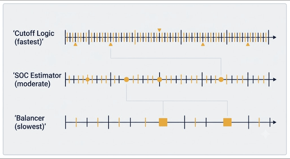
Sharing the right data at the wrong update rate still causes disagreement. The cutoff logic needs the fastest update path. A hard voltage limit can be reached in milliseconds, under a current spike. The SOC estimator can run on a slower cycle instead. Its correction task is inherently smoother. Design the shared state layer so each subsystem pulls at its own needed rate. Do not force one single rate onto all three.
How Subsystems Interact in an Integrated BMS Control Architecture
With shared state in place, the three subsystems can do more than avoid disagreement. They can actively support one another. The estimator’s SOC output can flag the balancer toward cells worth watching. The balancer’s voltage-spread data can flag the estimator when a cell’s behavior looks abnormal, rather than just imbalanced. The cutoff logic’s live DCIR reading, drawn from the same lookup table an EKF SOC estimation design pulls its resistance model from, keeps both systems working from one resistance picture instead of two.
Flagging Faults Instead of Silently Adapting
A well-built integrated BMS control architecture also creates a natural place to catch faults. If the shared DCIR reading from one cell departs sharply from its neighbors, and that departure does not track with the pack’s overall temperature or aging trend, the architecture can flag it as a possible fault, tied to the same in-service cell imbalance and DCIR drift patterns covered elsewhere in this series. This is far harder to catch when each subsystem only sees its own narrow slice of the picture.
Implementing an Integrated BMS Control Architecture Without a Full Redesign
For how centralized, modular, and wireless BMS topologies differ in where this shared layer can physically live, see our BMS architecture guide. Building an integrated BMS control architecture does not usually require new sensors. Most BMS hardware already measures voltage, current, and temperature at a resolution that supports this. The work is mostly in firmware: defining the shared data structure, setting update rates per subsystem, and routing each function’s calculation through the shared layer instead of an isolated local copy.
A Practical Migration Path
Start with the two subsystems most likely to disagree today: the SOC estimator and the cutoff logic, since both read current and voltage directly and both act on threshold logic. Confirm they draw from one shared, current-corrected voltage value before adding the balancer into the same layer. This staged approach limits the scope of any one firmware change and makes each step easier to validate on its own.
Key Takeaways
Three separate BMS modules can quietly disagree, even when each one works correctly on its own. An integrated BMS control architecture fixes this with one shared data layer for voltage, current, temperature, SOC, and DCIR, read by all three subsystems. Update timing matters as much as the shared data itself; each subsystem should pull at the rate its own task needs. Shared state also creates a natural place to flag developing faults, since a real fault shows up as one cell’s data breaking pattern against the rest of the shared picture.
Frequently Asked Questions
Does an integrated BMS control architecture need new hardware?
Usually not. Most BMS hardware already measures voltage, current, and temperature at a fine enough resolution. The work is mainly firmware: building a shared data layer and routing each subsystem’s calculation through it.
Which two subsystems should be integrated first?
Start with the SOC estimator and the cutoff logic. Both read current and voltage directly, and mismatches between them are the most likely to show up as a false or late cutoff trip.
How does an integrated BMS control architecture help catch developing faults?
When every subsystem shares one live view of each cell, a real fault shows up as that cell’s data breaking pattern against its neighbors and against the pack’s overall trend, rather than being missed by a subsystem that only sees its own narrow slice of the picture.
Cell matching before pack assembly sets a good starting point. But it does not stay good forever. In-service cell imbalance builds up over years. It builds long after the pack leaves the factory well matched. Heat, aging, and cycling all pull cells apart again. This guide covers the design choices that slow that drift. It covers thermal layout, balancing topology, and how imbalance control ties back into SOC estimation.
⚡ Quick Answer In-service cell imbalance grows mainly from two sources after assembly: uneven pack temperature, and the uneven aging that follows from it. Good thermal design and the right balancing topology both slow this drift. Neither one fixes a pack that started out badly matched.
Why In-Service Cell Imbalance Differs from Factory Mismatch
Factory cell matching solves the starting-point problem. Our cell matching before pack assembly guide covers that stage in depth. It groups cells by voltage, capacity, and resistance before assembly. In-service cell imbalance is a different, ongoing problem, however, because even a well-matched pack drifts apart over time. The BMS balances small gaps every cycle. But the size of that gap depends on design choices made outside the BMS itself.
The Feedback Loop Between Heat and Aging
This pattern matches published research on thermal gradients in lithium-ion packs, which found that uneven internal temperature drives inhomogeneous degradation and resistance growth well before a pack reaches end of life on paper. Heat is the main driver of in-service cell imbalance. A cell that runs hotter than its neighbors ages faster. It loses capacity faster and, as a result, it gains resistance faster too. Consequently, that resistance rise makes it sag more under load. More sag can make it run hotter still, at the same current. This is a feedback loop. Left unmanaged, a small temperature gap can grow into a real capacity gap. This can happen within a few years of daily cycling.
Designing Thermal Layout to Limit Imbalance
Thermal design is the first lever against in-service cell imbalance. It acts before the BMS ever needs to balance anything. For the specific causes of uneven pack temperature — coolant path position, cell position within the rack, and current-path resistance — and the ΔT targets a well-designed system should hit, see our cell temperature gradients guide. The takeaway for imbalance control specifically: any gradient beyond those targets does not just cost efficiency. It feeds directly into the heat-aging-resistance loop above, and the wider the gradient, the faster the affected cells pull away from the rest of the pack.
Design Around the Worst Case, Not the Average
A common mistake sizes cooling around the pack’s average temperature. Average temperature can look fine. Meanwhile, individual cells can sit well outside it. Measure the worst-case gradient across the pack instead of the mean. Design cooling around that number. This resistance rise is the same mechanism covered in our cell internal resistance guide. A pack running meaningfully above those ΔT targets — commonly the case in a poorly ventilated rack corner — is exactly the failure mode that accelerates in-service cell imbalance in the affected cells, over a multi-year service life.
Choosing a Balancing Topology for the Cycling Profile
Balancing topology is the second lever. Passive balancing bleeds excess energy off higher-SOC cells as heat. It is simple and low-cost. It works fine for light daily cycling with well-matched cells. But passive current is small. It is often just tens to a few hundred milliamps. It cannot keep pace with fast-building imbalance under heavy cycling or a strong thermal gradient.
Feature
Passive Balancing
Active Balancing
Typical current
Tens to a few hundred mA
1–5A
Cost
Low
Higher, more hardware
Best fit
Light daily cycling, well-matched cells
Heavy cycling, thermal gradients, long-duration assets
Energy handling
Bleeds excess as heat
Moves energy between cells
Effect on in-service cell imbalance
Slows drift on light-use systems
Keeps pace with faster-building drift
When Active Balancing Earns Its Cost Against In-Service Cell Imbalance
Active balancing moves energy between cells instead of burning it off. It corrects gaps far faster, at one to several amps. This higher cost pays off in three cases. First, systems that cycle more than once daily, since imbalance gets less rest time between corrections. Second, systems with a thermal gradient that design alone cannot remove — the same resistance growth this drives also affects cutoff timing; see our DCIR-adaptive cutoff guide. Third, long-duration systems built for fifteen years or more, where small ongoing gains add up to real lifetime value.
Linking Imbalance Back to SOC Estimation
In-service cell imbalance and SOC estimation accuracy feed each other. A design that treats them as separate problems will underperform. A biased SOC estimate can send the balancer a false signal. It might correct a gap that is not really there. Or it might miss one that is. This is the same shared-state problem seen in EKF SOC estimation design. The balancer and the estimator both need one current, shared view of each cell. They should not run on two readings that can quietly disagree.
Setting a Practical Alert Threshold
A voltage spread over 50 to 100 millivolts across cells is a common alert threshold on LFP. The chemistry’s flat curve means even a real SOC gap may show only a small voltage difference. Log these events instead of reacting to one reading. A single high-current moment can cause a spread that resolves on its own.
Key Takeaways
In-service cell imbalance differs from factory cell matching. It is driven mainly by heat, and the aging that heat speeds up. Thermal layout is the first line of defense, especially sizing cooling around worst-case gradients, not pack averages. Balancing topology should match the cycling profile. Passive balancing suits light daily cycling. Active balancing earns its cost in heavy-cycling, high-gradient, or long-duration systems. Imbalance control and SOC estimation should share state, not run as separate systems, since each one affects the accuracy of the other.
Frequently Asked Questions
What causes in-service cell imbalance if the pack started well matched?
Uneven pack temperature is the main driver. Hotter cells age faster and gain resistance faster. That raises sag under load, which can push the cell hotter still. The gap compounds over years of cycling.
Does active balancing fix a pack that started out mismatched?
No. Active balancing corrects ongoing in-service cell imbalance much faster than passive balancing. But neither approach can create capacity a weak cell never had. A bad starting mismatch still needs fixing at the cell-matching stage, before assembly.
What voltage spread signals a real in-service cell imbalance problem on LFP?
A spread over 50 to 100 millivolts is a common threshold worth checking. Still, the trend across cycles matters more than any single reading.
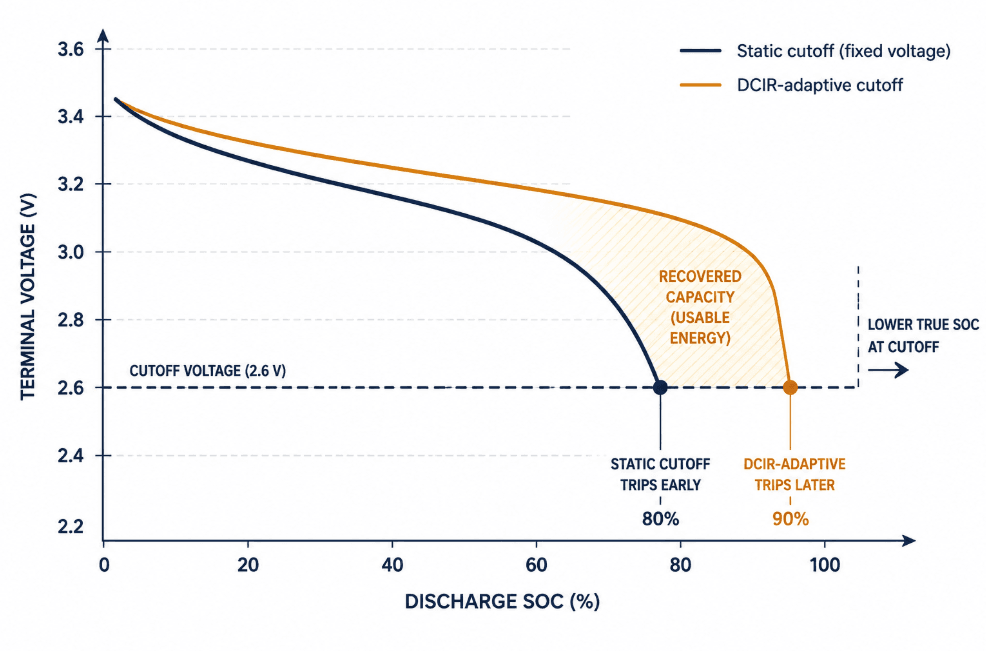
A static low-voltage cutoff pulls one fixed value from a cell datasheet. That single number is one of the most common reasons a BESS underdelivers its rated usable capacity. As direct current internal resistance (DCIR) rises with cell age, it also rises as temperature drops. The voltage sag under load grows along with it. A fixed cutoff trips earlier and earlier in the discharge curve, even though the cell still has real, recoverable capacity left. This article walks through how to design a DCIR-adaptive cutoff instead. It covers the test data it requires, the lookup-table structure a BMS actually implements, and the throughput recovered as a result.
⚡ Quick Answer A DCIR-adaptive cutoff replaces one fixed trip voltage with a value calculated in real time. It pulls current and a resistance value from an HPPC-derived lookup table, indexed by SOC, temperature, and cell age. This raises the effective cutoff trigger to match present-moment resistance, instead of a fresh-cell assumption — recovering up to 10% of effective throughput in mid-to-late project life that a static cutoff would otherwise strand.
Why a Fixed Cutoff Voltage Is the Wrong Design Choice
A discharge cutoff exists to stop the pack before any cell drops below its safe minimum voltage — commonly 2.5V per cell for LFP. The problem is where that voltage gets measured. Terminal voltage under load equals open-circuit voltage minus the resistive sag: V(terminal) = V(OCV) − I × DCIR. A fresh cell with 0.15 mΩ DCIR sags very little even at high current. The same cell after several thousand cycles sags far more. Its DCIR has risen to 0.3–0.5 mΩ, and it sags two to three times as much at identical current. So the BMS reaches the 2.5V trip point at a meaningfully higher residual state of charge, even though the cell’s actual OCV-based SOC has not changed.
Temperature compounds this effect further. Internal resistance rises sharply as cell temperature falls. Ion mobility slows down in the cold, both in the electrolyte and at the electrode interface. A cutoff threshold validated only at 25°C on a fresh cell will trip early on both counts, in a cold, aged pack. Sometimes this strands 10–15% of nameplate capacity that the cell was never actually short of.
Building the DCIR-SOC-Temperature Map for a DCIR-Adaptive Cutoff
The data foundation for a DCIR-adaptive cutoff is Hybrid Pulse Power Characterization (HPPC) testing. This methodology was developed under the US Department of Energy’s USABC/PNGV programs. It is now standard practice across automotive and stationary storage cell qualification. HPPC applies paired discharge and charge current pulses at fixed SOC steps, typically every 10% of capacity. It runs this across a matrix of test temperatures, and measures the resulting voltage response to extract resistance at each point. This is the same underlying test data an EKF SOC estimation design uses to build its own equivalent circuit model. A project running one HPPC campaign can feed both efforts from a single test matrix.
Discharge the cell to each target SOC step and allow it to rest until voltage stabilizes.
Apply a short current pulse (commonly 10 seconds) at the rated or peak discharge current and record the instantaneous voltage drop.
Calculate DCIR at that SOC and temperature as ΔV divided by the pulse current.
Repeat across the full SOC range and across a temperature matrix spanning the system’s expected operating envelope, from cold-climate minimums to peak ambient.
Repeat the full test periodically through a cycle-aging program to capture how the resistance surface shifts with cell age, not just with SOC and temperature.
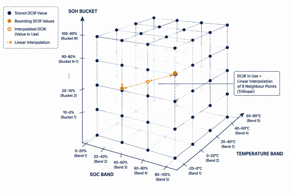
The output is a three-dimensional resistance surface — DCIR as a function of SOC, temperature, and cycle count or SOH — rather than a single number. This surface is what the BMS firmware references at runtime instead of a fixed cutoff voltage.
From Resistance Surface to a DCIR-Adaptive Cutoff Lookup Table
Translating HPPC data into a working DCIR-adaptive cutoff requires converting the continuous resistance surface into a discrete lookup table. This table has to be one the firmware can query in real time, without heavy onboard computation.
Structuring the Lookup Table
A practical implementation follows this structure:
Index the table by SOC band (e.g., 10% steps), temperature band (e.g., 5°C steps), and a coarse SOH bucket (e.g., every 500–1,000 cycles or a measured capacity-fade threshold).
Store a DCIR value at each grid point, interpolating linearly between points at runtime rather than storing every possible combination.
Calculate the adjusted cutoff voltage in real time as V(cutoff, adjusted) = V(cutoff, minimum) + I(measured) × DCIR(SOC, T, SOH) — raising the effective cutoff trigger point to reflect present-moment resistance rather than a static assumption.
Apply hysteresis around the cutoff transition to prevent the BMS from oscillating between discharge-enabled and discharge-disabled states as current and resistance fluctuate near the boundary.
Re-anchor the SOH bucket periodically using either a full capacity test or a DCIR-trend proxy, since resistance growth is one of the standard leading indicators for SOH estimation without requiring a full discharge test.
Using resistance trend as an SOH proxy rather than running a full capacity test lines up with current battery-health research: a recent review of experimental health-assessment methods for lithium-ion cells names pulse-based resistance testing among the practical indicators for tracking degradation without the time and equipment cost of a full discharge cycle.
How Static and DCIR-Adaptive Cutoffs Compare
Reference point
Single fixed voltage from cell datasheet
Real-time calculated voltage adjusted for measured current × DCIR
Temperature handling
Assumes room-temperature test conditions
Indexed by temperature band from HPPC matrix
Aging handling
Fixed for asset life
Indexed by SOH bucket; re-anchored periodically
Typical result at 1C, mid-to-late project life
10–15% of nameplate capacity stranded
Recovers up to 10% of effective throughput
Data source
Cell datasheet single-point spec
HPPC test matrix across SOC × temperature × cycle count
Where the Recovered Throughput Comes From
The revenue case for this design change is straightforward. DCIR-driven voltage sag can shrink the usable SOC window by roughly 10–15% in mid-to-late project life, at high C-rates. Our 0.5C vs 1C cycle life analysis puts a number on the recoverable share of that: a DCIR-adaptive cutoff recovers up to 10% of effective throughput in mid-to-late project life. It does this by letting discharge continue closer to the cell’s true low-SOC limit, rather than tripping on resistance alone. Over a multi-year asset life, this compounds. Every cycle that discharges 10% deeper than a static cutoff would have allowed is 10% more throughput on that cycle. Multiply that across thousands of cycles. For dispatch-contracted or market-facing assets, this also improves bid accuracy. The state-of-charge and state-of-power figures reported to the EMS more closely match what the pack can actually deliver under load.
Implementation Notes and Common Pitfalls
Don’t confuse SOC estimation with cutoff calibration
A DCIR-adaptive cutoff corrects for resistance-driven voltage sag; it does not replace the underlying SOC estimation algorithm. An accurate EKF-based SOC estimate can still trip early under load if the cutoff voltage itself is static. Both layers need attention. For the estimation side of this problem, including how a biased SOC output can itself shift where a DCIR-adaptive cutoff trips, see our EKF SOC estimation design guide. SOC estimation accuracy and cutoff voltage adaptivity solve different problems that happen to share the same root cause in LFP’s flat OCV curve.
Validate That the DCIR-Adaptive Cutoff Doesn’t Mask Genuine Cell Faults
A DCIR-adaptive cutoff must still tell apart two different things. One is normal, predictable resistance growth. The other is an abnormal resistance spike from a developing fault — a loose busbar connection, a failing weld, or accelerated local aging tied to in-service cell imbalance. Cross-check measured DCIR against the expected value from the lookup table, rather than blindly applying the adjustment. This lets the BMS flag anomalies instead of quietly adapting around them.
Size cooling and current limits around end-of-life DCIR, not fresh-cell DCIR
The same resistance surface that feeds the cutoff table should also inform thermal design margin and current-limiting logic. Heat generation scales with resistance and the square of current. Designing cooling capacity around fresh-cell impedance under-sizes the system for the DCIR it will actually see in year eight or ten. None of these three systems — cutoff logic, SOC estimation, and imbalance control — should run as fully isolated modules. Our integrated BMS control architecture guide covers how to share DCIR, current, and temperature state across all three.
Key Takeaways
A fixed low-voltage cutoff ignores the fact that DCIR rises with both cell age and cold temperature, which strands usable capacity that the pack technically still has. HPPC testing across a SOC × temperature × cycle-count matrix is the standard method for building the resistance data a DCIR-adaptive cutoff needs. The firmware implementation is a lookup table with linear interpolation, not a continuous real-time model — this keeps the calculation lightweight enough for BMS hardware. A DCIR-adaptive cutoff recovers up to 10% of effective throughput in mid-to-late project life, most of the capacity that would otherwise sit stranded behind a static, resistance-blind trip point. Cutoff adaptivity and SOC estimation accuracy are separate problems. Both trace back to LFP’s flat voltage curve. Fixing one does not fix the other.
Frequently Asked Questions
Is a DCIR-adaptive cutoff a firmware-only change, or does it require new hardware?
In most cases it is a firmware and calibration-data change rather than a hardware change, provided the BMS already measures cell voltage and pack current with sufficient resolution and sampling rate. The work is in generating the HPPC-derived lookup table and implementing the interpolation and hysteresis logic, not in adding sensors.
How often does the resistance lookup table need to be re-validated?
A practical cadence ties re-validation to SOH milestones rather than a fixed calendar interval — for example, every 500–1,000 cycles or whenever a capacity or DCIR trend crosses a defined threshold. Systems with continuous DCIR trending can trigger table updates automatically rather than requiring a manual test campaign.
Does a DCIR-adaptive cutoff increase the risk of over-discharging a cell?
No, when implemented correctly. The adjustment raises the effective cutoff trigger voltage to compensate for load-induced sag. It does not lower the cell’s true minimum safe voltage. That real, OCV-based SOC is still where the cell trips. The BMS is simply better at recognizing where that point is under load, instead of confusing resistive sag for depleted charge.
References
• HPPC Test Procedure — Hybrid Pulse Power Characterisation methodology originating from the USABC/PNGV development program.
Every BESS reports a state of charge number to its EMS. That number drives dispatch. It drives revenue. It drives warranty math too. Good EKF SOC estimation design keeps that number honest. It stays honest even as cells age. It stays honest as temperatures shift and load patterns change. This guide covers steps most SOC articles skip. First, build the model. Then fit it from test data. Then tune the filter so it corrects errors fast, without chasing sensor noise.
⚡ Quick Answer EKF SOC estimation design means building a circuit model of the cell from HPPC test data, then tuning the Kalman filter so it trusts the model at rest and trusts the sensors under load. Get the model wrong, or the tuning wrong, and the filter either drifts like open-loop counting or jumps around on every current spike.
From HPPC Data to an Equivalent Circuit Model
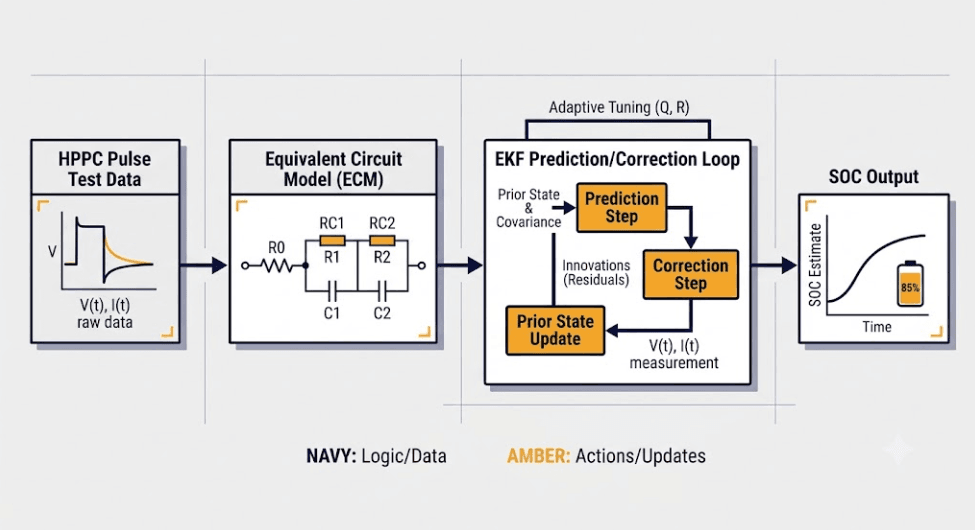
An EKF cannot estimate what it cannot model. So the first step in EKF SOC estimation design is building an equivalent circuit model, or ECM. This model describes how terminal voltage responds to current. A simple, first-order ECM uses three parts: an open-circuit voltage source, a series resistance, and one resistor-capacitor pair for voltage relaxation. Many BESS projects use a second-order ECM instead. That adds a second RC pair. It separates fast charge-transfer effects from slower diffusion effects.
Extracting Parameters from Pulse Data for EKF SOC Estimation Design
HPPC testing supplies the raw data for this step. It is the same pulse-and-rest method used to build a DCIR lookup table for a dynamic cutoff. Each pulse reveals resistance from the instant voltage step. It reveals RC time constants from the relaxation curve after. Good EKF SOC estimation design fits these parameters at every SOC and temperature step in the test matrix. Do not fit just once at a nominal point. LFP’s resistance shifts across the full range, and so does its relaxation behavior.
Why the Flat OCV Curve Still Matters
LFP’s OCV-SOC curve is flat between 20% and 80%. This is why Coulomb counting and OCV lookup drift on their own. It is also why EKF SOC estimation design must treat the OCV-SOC table as a core model input, not an afterthought. A weak OCV curve in the flat zone gives the filter almost nothing to correct against, right where correction matters most.
Tuning the Filter: The Core of EKF SOC Estimation Design
This filtering approach builds on the adaptive extended Kalman filter method for battery state estimation, adapted here specifically for LFP’s flat OCV-SOC curve. For the three underlying SOC methods this design builds on, our BMS SOC estimation methods guide covers OCV lookup, Coulomb counting, and Kalman filtering at a conceptual level. Once the ECM exists, the filter itself needs tuning. Two settings control its behavior. Process noise covariance, called Q, sets how much the filter trusts its own model between updates. Measurement noise covariance, called R, sets how much it trusts each voltage reading. Together, these two numbers set the correction strength. This step is the heart of real EKF SOC estimation design work.
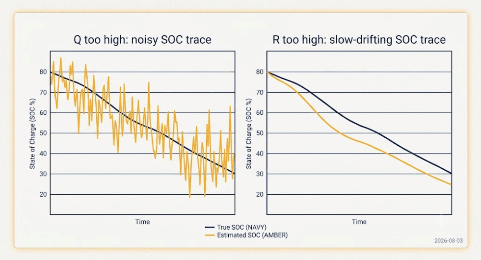
What Happens When Q Is Too High
A high Q value tells the filter its model cannot be trusted. So it leans hard on every voltage sample instead. But on LFP’s flat curve, that sample carries almost no SOC signal across most of the range. The estimate turns noisy and jumpy during normal cycling. This is a common failure. The filter looks fine on a bench test. Then it behaves badly once deployed against real load profiles.
What Happens When R Is Too High
The opposite mistake sets R too high. That tells the filter to distrust the voltage reading. The estimate then acts like open-loop Coulomb counting. It drifts slowly over days, since it never truly corrects against sensor data. Both mistakes produce the same bad outcome: a confident but wrong SOC number. That is worse for dispatch accuracy than a system that visibly struggles.
A Practical Starting Point for Tuning
Start Q and R from real numbers. Use your measured sensor noise floor. Use your HPPC fit residuals. Then adjust by testing against a validation cycle the model has not seen before. An adaptive approach helps too. Let R scale up automatically during high-current transients, when voltage sag dominates the signal. This improves robustness without manual retuning for every duty cycle.
Where Estimation Error Spreads to the Other Two Problems
EKF SOC estimation design does not stand alone. A biased estimate feeds two other systems directly. First, it distorts the balancer’s target. If the estimator reports a false high SOC on one cell, the balancer under-corrects a real gap, and that gap grows — see our in-service cell imbalance guide for how that plays out at the pack level. Second, it distorts cutoff logic. For the full LFP-specific voltage and temperature parameters this estimator design has to respect, see our BMS for LiFePO4 batteries guide. A DCIR-adaptive cutoff uses the same current and temperature inputs the estimator uses. A wrong SOC estimate near empty can trigger a cutoff too early, or too late, relative to the cell’s true state.
This is why SOC estimation belongs beside cell balancing and cutoff design, not as a separate topic on its own. The three systems share inputs. In a well-built BMS, they should share state too, not run as separate, disconnected modules— our integrated BMS control architecture guide covers how to build that shared state layer.
Validating EKF SOC Estimation Design Before Deployment
EKF SOC estimation design is not finished once tuning looks good on paper. Before field deployment, test the tuned filter against a real dispatch profile. Do not just replay the HPPC pulse sequence. A filter can track a clean pulse test well, then still fail on a real profile full of irregular current swings. At the end of validation, compare the filter’s estimate against a full charge-discharge cycle. That full cycle gives a true anchor point. The filter’s own reported error cannot hide from it.
Re-Validating EKF SOC Estimation Design as Cells Age
ECM parameters from beginning of life will not hold for the system’s full service life. Resistance grows. Capacity fades. So the same periodic HPPC re-test that refreshes a DCIR-adaptive cutoff table should also refresh the EKF’s model. Tie both refresh cycles to one shared SOH milestone. That keeps the estimator and the cutoff logic working from the same, current view of the pack.
Key Takeaways
EKF SOC estimation design starts with a circuit model fitted from HPPC pulse data, across the full SOC and temperature matrix. Process and measurement covariance tuning decides whether the filter trusts its model or its sensors, and getting either one wrong produces a noisy or a slow-drifting estimate. SOC estimation error never stays contained. It spreads into balancing decisions and cutoff timing too. Re-validate the model often, on the same schedule as other resistance-based BMS recalibrations.
Frequently Asked Questions
Does EKF SOC estimation design need a first-order or second-order model for LFP?
A second-order model captures LFP’s diffusion behavior more accurately. It is standard for utility-scale and precision work. A first-order model is lighter on BMS processing budget. It can be enough for smaller residential systems with lighter accuracy needs.
How often should the EKF model be re-tuned?
Tie re-tuning to the same SOH milestone used for other resistance-based recalibrations. That is commonly every 500 to 1,000 cycles, or whenever a capacity or resistance trend crosses a set threshold, rather than a fixed calendar date.
Can a poorly tuned EKF cause a false cutoff trip?
Yes. A dynamic cutoff calculates its trip voltage from the same current and modeled resistance the estimator uses. So a biased SOC estimate near empty can shift the effective cutoff point away from the cell’s true safe limit.
⚡ Quick Answer: Cell Internal Resistance in Brief Cell internal resistance is the opposition a lithium-ion cell presents to current flow. It combines ohmic resistance (foils, tabs, electrolyte), charge-transfer polarization (the reaction barrier at the electrode surface), and diffusion polarization (ion movement inside the electrode). It is measured in milliohms, rises with age, cold temperature, and extreme state of charge, and directly governs heat generation, round-trip efficiency, and available power. ACIR, DCIR, and EIS are the three standard ways to measure it.
What Is Cell Internal Resistance?
Every lithium-ion cell acts like a small resistor. It sits in series with an ideal voltage source. So when current flows, part of the cell’s energy turns into heat. It never reaches the terminals as usable power. This loss is called cell internal resistance, or Cell IR for short.
Cell IR is not one single part. Instead, it is a combined value. It captures several resistive and electrochemical processes happening at once. As a result, Cell IR changes with temperature, state of charge (SOC), and age. In fact, this is also why two test methods, ACIR and DCIR, can report different numbers for the same cell.
Current-collector foils, tabs, weld joints, separator, and electrolyte conductivity — a true, frequency-independent resistance
Instantaneous; measured directly by 1 kHz ACIR
Charge-transfer (activation) polarization
The energy barrier lithium ions must overcome to cross the electrode–electrolyte interface
Milliseconds to seconds into a current pulse
Diffusion (concentration) polarization
Ion movement and concentration gradients inside the solid electrode particles and electrolyte
Seconds to minutes; dominant during sustained load
Ohmic resistance responds right away. Diffusion resistance, by contrast, builds up slowly over time. So the length of the test pulse changes what you actually measure. That, in short, is why a 1 kHz ACIR reading and a multi-second DCIR pulse test rarely agree on the same cell.
Key Takeaways: Cell Internal Resistance at a Glance
Attribute
Summary
Typical unit
Milliohms (mΩ) for large-format cells; the value scales with electrode/tab area, so small cylindrical cells read much higher than large prismatic cells
Large-format LFP prismatic cells (280–314 Ah)
Commonly 0.15–0.5 mΩ ACIR at 1 kHz, 25 °C, ~30% SOC, varying by manufacturer and grade
Primary heat mechanism
Joule heating, P = I²R — heat rises with the square of current
Rises with
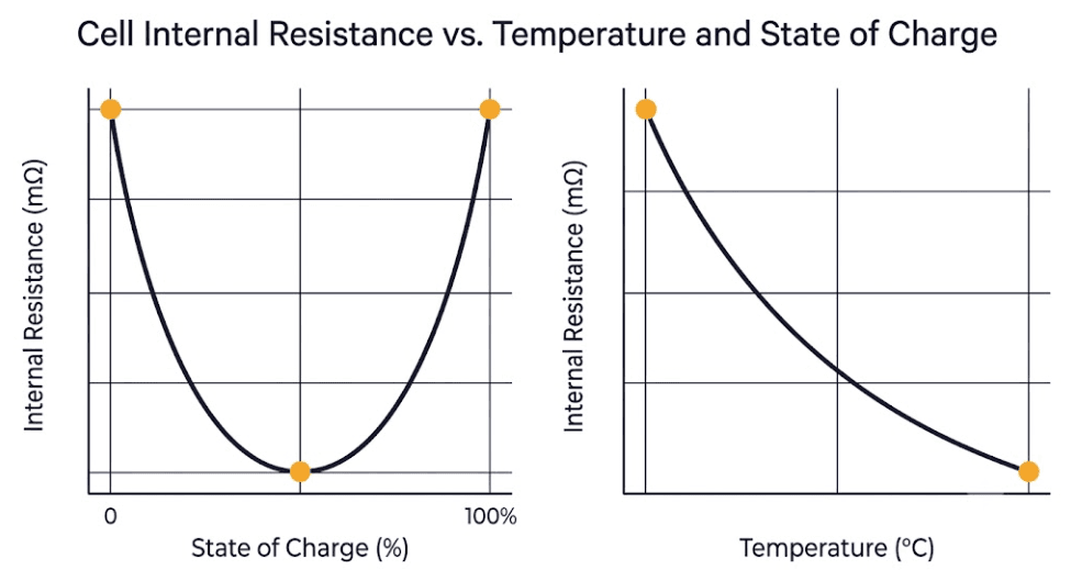
Cell aging/cycling, cold temperature, and SOC extremes (very low or very high)
Lowest at
Mid-range SOC (roughly 30–70%) and moderate temperature (roughly 15–35 °C)
Standard measurement methods
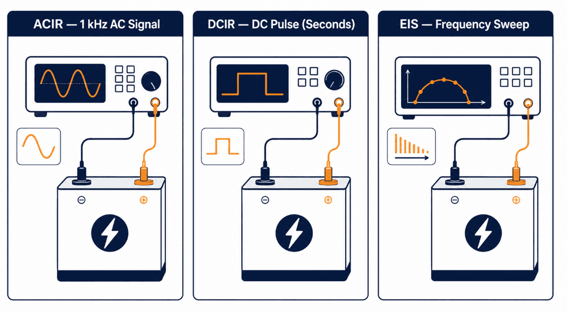
ACIR (1 kHz AC), DCIR (DC pulse), EIS (frequency sweep)
Cell IR is the main source of heat inside an operating cell. Heat generation follows Joule’s law: P = I²R. In other words, heat rises with the square of current. So, even a small increase in resistance causes a large rise in thermal load at high C-rates. That is why, in practice, BESS designers usually size cooling systems around worst-case DCIR rather than nameplate ACIR.
2. Cell IR and Round-Trip Efficiency
Every milliohm of resistance turns some charge and discharge energy into waste heat. This happens instead of usable throughput. Consequently, this resistive loss is one of the main contributors to round-trip efficiency. It sits alongside power-conversion and thermal-management losses.
3. Cell IR, Available Power, and Voltage Sag
Under high current draw, resistance causes the terminal voltage to sag below the open-circuit voltage. If resistance is high enough, that sag can push the terminal voltage below an inverter’s cutoff threshold. This can happen even while real charge remains in the cell. In practice, then, it is a nuisance trip that looks like a capacity problem. In fact, it is a resistance problem.
4. Cell IR as a Leading Indicator of Aging
Cell IR, particularly DCIR, tends to rise before rated capacity visibly degrades. As the solid-electrolyte interphase (SEI) layer thickens with cycling, resistance climbs steadily. For this reason, resistance tracking is a standard input to State of Health (SOH) estimation.
What Changes Cell Internal Resistance
Cell IR is not a fixed number on a datasheet. Instead, it is a dynamic value that shifts with operating conditions. So, the factors below explain most of the variation seen in the field.
Factor
Effect on Internal Resistance
Temperature
Resistance falls as temperature rises (faster ion mobility) and climbs sharply below roughly 0 °C; temperature swings of ±10 °C can shift measured resistance by around 20%
State of charge (SOC)
Follows a U-shaped curve — lowest in the mid-SOC range, rising again at very high and especially very low SOC as diffusion polarization increases
Aging / cycle count
Rises steadily over cell life as the SEI layer thickens and active material loses contact; DCIR growth of roughly 50–150% over a cell’s usable life is commonly reported, with LFP tending to show faster proportional resistance growth than NMC
C-rate / pulse duration
Longer, higher-current pulses capture more diffusion polarization, so DCIR measured over several seconds reads higher than a short 1 kHz ACIR snapshot on the same cell
Cell format and design
Large-format prismatic and pouch cells generally report lower resistance per cell than small cylindrical formats, because tab and current-collector area — not just chemistry — governs the ohmic term
Manufacturing quality / grade
Electrode coating uniformity, electrolyte wetting, and weld quality all shift the ohmic term; grading by resistance is a standard incoming-QC step for large-format LFP cells
#image_title
Cell Internal Resistance: LFP vs. Other Chemistries
Lithium iron phosphate (LFP) cells usually start life with low, stable resistance. This is true compared with nickel-based chemistries. In fact, it is one reason LFP has become the default choice for stationary BESS. However, field research on LFP cell aging shows resistance growth speeds up faster, in relative terms, than in NMC cells as cycling progresses. As a result, resistance trending is a more important monitoring parameter for LFP-based systems over a 10–15 year project life. For a full chemistry-level safety comparison, meanwhile, see NMC Battery vs LFP Safety: The Complete BESS Risk Breakdown.
How Cell Internal Resistance Is Measured
Three methods dominate industrial and BESS-integrator practice. Each one, however, answers a slightly different question. So this section compares all three, to help you choose the right one.
Method
Signal Type
What It Captures
Typical Use
ACIR
Small AC current at 1 kHz
Ohmic resistance only — fast, repeatable, standardized
Incoming cell QC, sorting, and grading
DCIR
DC current step or pulse (seconds)
Ohmic + charge-transfer + diffusion polarization together
System-level power modeling, thermal design, real-world performance
EIS
AC sweep from mHz to tens of kHz
Separates all three components individually across frequency
ACIR is fast, taking under a second per cell. It is also highly repeatable. For this reason, it is the standard tool for grading incoming cells at the factory. DCIR, on the other hand, takes longer. But it reflects how a cell actually behaves under a real grid-power pulse. Therefore, it is the preferred input for thermal and power-delivery modeling, as Keysight’s ACIR and DCIR measurement methodology explains. EIS, meanwhile, is the slowest and most instrument-intensive method. So it is reserved for diagnostic work, where engineers need to know exactly which resistance component is degrading.
Cells assembled into a series string should be matched on capacity and open-circuit voltage. However, they should also be matched on Cell IR. A cell with much higher resistance than its neighbors heats faster and sags further under load. It also drifts out of SOC balance faster. This, in turn, speeds up imbalance, even when the BMS works correctly.
Cell IR and Thermal Design Margin
Heat scales with resistance and the square of current. Therefore, thermal designers size cooling capacity around worst-case DCIR at end-of-life, not fresh-cell ACIR. Ignoring resistance growth over the warranty period, unfortunately, is a common cause of undersized thermal margin in early-life system designs.
SOH Estimation and Voltage-Sag Protection
DCIR climbs in a predictable way with age. Because of this, it is one of the standard inputs a BMS uses to estimate State of Health without a full capacity test. Resistance data, in addition, informs voltage-sag-aware cutoff thresholds. In turn, this prevents the BMS from tripping early on a cell that still has usable charge but momentarily high resistance under load.
Frequently Asked Questions
What is a normal cell internal resistance for a LiFePO4 cell?
It depends heavily on cell size. Large-format prismatic LFP cells used in BESS (280–314 Ah) typically measure around 0.15–0.5 mΩ ACIR at 25 °C and roughly 30% SOC. This, of course, varies by manufacturer and grade. Smaller cylindrical LFP cells, by contrast, have much less current-collector and tab area. So they commonly measure in the tens of milliohms.
Does cell internal resistance always increase with age?
In normal operation, yes. Resistance trends upward over a cell’s cycle life as the SEI layer thickens and internal contact degrades. However, the rate varies by chemistry, temperature history, and depth of discharge. Notably, a sudden, sharp resistance spike, rather than a gradual trend, is more likely to signal a fault than normal aging.
Why does Cell IR increase in cold weather?
Low temperature slows lithium-ion movement in the electrolyte. It also slows the electrochemical reactions at the electrode surface. Together, these effects raise both the ohmic and polarization parts of resistance. This is why cold-climate BESS enclosures use insulation and heating elements. As a result, cells stay within their optimal temperature band before drawing high power.
Is lower resistance always better?
Lower resistance generally means less heat, higher efficiency, and more available power. However, resistance is only one design variable among several. Some manufacturers, in fact, accept a modest resistance trade-off for a formulation that prioritizes thermal stability or cycle life. Overall, then, resistance should be evaluated alongside safety margin and cycle-life data, not in isolation.
Is ACIR or DCIR more accurate?
Neither is universally more accurate; they simply answer different questions. ACIR is the more repeatable, standardized snapshot of ohmic resistance. So it works best for comparing cells to each other. DCIR, on the other hand, reflects how the cell behaves under an actual power pulse. This, in turn, makes it the better input for system-level thermal and performance modeling.
Power outages cost businesses billions every year. Aging grid infrastructure, extreme weather, and the variable nature of solar and wind energy make centralized power systems less reliable. As a result, energy-forward organizations are turning to microgrid BESS — a combination of distributed energy resources and battery storage that can supply power independently of the utility grid.
A microgrid BESS is not simply a backup generator. Instead, it is an intelligent energy platform that stores renewable energy, dispatches it on demand, and switches smoothly between grid-connected and islanded operation. To understand the foundation of this technology, read our ultimate guide to battery energy storage systems before diving into the microgrid-specific details covered here.
This guide covers everything EPCs, project developers, and commercial energy buyers need to know. Topics include: how these systems work, core components, sizing methodology, use cases, grid-forming technology, relevant standards, and financial considerations.
What Is a Microgrid BESS?
A microgrid is a local energy network. It integrates distributed energy resources — solar PV, wind turbines, diesel generators, and battery storage — into one controllable system. Crucially, it can run in two modes: grid-connected (exchanging power with the utility) or islanded (supplying loads on its own).
Battery storage is the technology that makes islanded operation practical. Without BESS, a microgrid relying on solar cannot guarantee stable voltage and frequency when it disconnects from the grid. With BESS, however, the system buffers generation gaps, sustains loads overnight, and holds the frequency reference that other devices need. For a broader look at how BESS works across sectors, see our guide on top applications of commercial and industrial BESS.
In short: BESS is the backbone of a modern microgrid. It turns a set of distributed generators into a self-sufficient power system.
Grid-Connected vs. Islanded Microgrid BESS
Microgrid BESS Operating Modes — Grid-Connected vs. Islanded
Microgrid BESS operates in two fundamental modes. Understanding both is essential before sizing or specifying a system.
Grid-connected mode: The microgrid stays synchronized with the utility. BESS handles peak shaving, load shifting, and frequency regulation. Excess solar generation is stored or exported.
Islanded (off-grid) mode: The microgrid disconnects at the point of common coupling. BESS then acts as the voltage reference, sustaining all local loads entirely on its own.
Seamless transition between these modes is a critical performance target. Research published in Energies (2026) showed loss-of-mains detection in under 3 milliseconds — well within the 10-millisecond threshold needed for sensitive equipment to ride through without disruption.
Core Components of a Microgrid BESS System
A complete microgrid BESS integrates several interdependent subsystems. Knowing each one helps EPCs design reliable systems and helps project developers evaluate vendor proposals accurately.
1. Battery Modules and Racks — LFP Chemistry
Lithium Iron Phosphate (LFP) chemistry dominates microgrid deployments today. LFP delivers over 6,000 cycles at 80% depth of discharge. It also operates safely across wide temperature ranges and avoids the thermal runaway risk seen in NMC chemistry. Battery modules are assembled into racks and housed in containerized enclosures for rapid site deployment.
2. Battery Management System (BMS)
The BMS monitors cell-level voltage, temperature, and current. It enforces SoC limits (typically 20–80% under the 20/80 cycling rule), calculates State of Health (SoH), and tracks DC Internal Resistance (DCIR). Additionally, the BMS communicates with the EMS via CAN bus or Modbus. For a deeper look at how the EMS works inside a BESS, we have a dedicated technical article on the subject.
3. Power Conversion System (PCS)
The PCS — also called the bidirectional inverter — converts DC energy from batteries into AC power for loads. It also converts AC to DC during charging. In a microgrid, the PCS can operate in grid-following or grid-forming mode. Grid-forming units synthesize voltage and frequency from scratch, which makes islanded operation possible even without a utility reference.
4. Energy Management System (EMS)
The EMS is the intelligence layer. It receives data from the BMS, PCS, solar inverters, load meters, and weather forecasts. Then it dispatches charge/discharge commands to optimize across multiple objectives simultaneously — peak shaving, renewable self-consumption, SoC management, and grid services. Moreover, it governs mode transitions and coordinates load shedding during generation shortfalls. Read our full breakdown of how EMS enables advanced grid services through BESS to see exactly how this works in practice.
5. Solar PV Array
Solar PV is the primary generation source in most microgrid BESS deployments. The PV array charges the BESS during daylight hours. As a result, the BESS can supply loads through the night or during cloud cover. Oversizing the PV-to-BESS ratio — typically 1.2× to 1.5× — ensures adequate charging under real-world irradiance conditions.
6. Point of Common Coupling (PCC) Switch / STS
The PCC switch or Static Transfer Switch (STS) is the electrical boundary between the microgrid and the utility grid. During a grid disturbance, the STS opens within milliseconds to island the microgrid. When grid power returns and stabilizes, the STS synchronizes and re-closes. Consequently, the speed and reliability of this device directly determines the quality of power continuity during transitions.
Microgrid BESS Component Summary Table
Component
Primary Function
Key Standard
Typical Technology
Battery Module
Store DC energy
IEC 62619, UL 1973
LFP, NMC
BMS
Cell monitoring, protection, SoH tracking
IEC 62133-2
Rack-level + pack-level
PCS / Inverter
DC↔AC conversion, grid forming/following
IEEE 1547, UL 1741
Grid-forming (VSM/droop)
EMS
Dispatch, optimization, mode transitions
IEC 62933-5-2
SCADA + AI forecasting
STS / PCC Switch
Grid isolation, mode transition
IEEE 1547.4
<20 ms transfer
Solar PV Array
Primary renewable generation
IEC 61215, IEC 61730
Monocrystalline TOPCon
Thermal Management
Temperature control, fire suppression
NFPA 855, UL 9540A
HVAC + liquid cooling
Microgrid BESS Components Architecture Diagram
Grid-Forming BESS: The Key to True Islanding
The most important technology choice in any microgrid BESS project is the inverter control mode. Specifically, you must decide between grid-following and grid-forming. This single decision determines whether the system can operate independently of the utility at all. Our detailed grid-forming vs. grid-following BESS guide covers the full technical comparison, but the key points are summarized below.
Grid-Following BESS: Its Core Limitation
A grid-following inverter acts as a current source. It detects the voltage and frequency of an active grid and synchronizes its output to that reference. Therefore, if the grid disappears — during a blackout — a grid-following inverter cannot sustain islanded operation. It must shut down immediately per IEEE 1547 anti-islanding requirements to protect utility workers.
This means a grid-following BESS cannot black-start a dead network. Nor can it sustain an islanded microgrid on its own. As a result, it is not a viable standalone solution for resilience-critical sites.
Grid-Forming BESS: How It Creates the Grid
Grid-Forming vs Grid-Following BESS Inverter Comparison
A grid-forming inverter operates as a voltage source instead. Rather than following an external signal, it synthesizes its own voltage waveform and frequency using algorithms such as Virtual Synchronous Machine (VSM) or droop control. Consequently, all devices on the microgrid — other inverters, loads, generators — synchronize to the grid-forming BESS.
This fundamental shift in control architecture unlocks four critical capabilities:
Black start: The grid-forming BESS energizes a completely dead network from zero.
Sustained islanding: The microgrid runs indefinitely without any utility connection.
Synthetic inertia: The inverter emulates the rotational inertia of a synchronous generator, stabilizing frequency during rapid load changes.
Fault current contribution: The system provides enough fault current to trip protection relays, enabling conventional protection coordination.
As of mid-2025, Australia had deployed 1,070 MW of grid-forming BESS across ten sites, according to AEMO. Furthermore, a 2025 Nature Scientific Reports study confirmed that integrated grid-forming inverter strategies significantly improve microgrid resilience under fault conditions. This real-world track record proves that grid-forming technology is no longer experimental.
How to Size a Microgrid BESSSystem
Getting the size right is critical. An undersized system fails to cover loads overnight or during weather events. An oversized system wastes capital. Fortunately, the sizing methodology follows four clear, sequential steps.
Step 1 — Establish the Load Profile
Start with a complete energy audit. Measure peak demand (kW) and daily energy consumption (kWh). Identify critical loads that must run during islanding and non-critical loads that can be shed. Also account for motor start-up inrush currents, which can reach 6× running current and must be covered by the PCS peak power rating.
Step 2 — Define Autonomy Duration
Autonomy duration is the number of hours the microgrid must sustain critical loads without solar generation or grid support. For most commercial microgrids, 4–8 hours covers overnight periods. For resilience-critical facilities such as hospitals or data centers, however, 24–72 hours of autonomy is the standard design target.
Step 3 — Apply the Sizing Formula
Use this baseline formula to calculate required battery capacity:
Here: DoD = usable depth of discharge (0.80 for LFP); RTE = round-trip efficiency (0.92 for modern LFP BESS). Always add a 10–15% spinning reserve margin on top for frequency stability headroom.
Step 4 — Size the Solar PV Array
The solar PV array must fully recharge the BESS within the available daylight window. For a system that recharges overnight-depleted batteries within 6–8 hours of sunlight, a PV-to-BESS ratio of 1.3× to 1.5× is typically required. NREL’s battery storage FAQs provide reliable guidance on irradiance-based sizing methodology that you can apply directly to project scoping.
Microgrid BESS Sizing Reference Table
The table below assumes LFP chemistry, 80% DoD, 92% RTE, 10% spinning reserve, and 12-hour overnight autonomy:
Application
Critical Load (kW)
Autonomy (h)
BESS Size (kWh)
Solar PV (kWp)
Remote Village
50
12
817
1,060
Commercial Campus
250
8
2,717
3,500
Hospital / Critical Site
500
24
16,304
21,000
Mining / Industrial
1,000
12
16,304
21,000
Island Community
2,000
12
32,609
42,000
Note: These are scoping figures only. Final sizing must account for site-specific irradiance, load diversity factor, planned expansion, and local grid code requirements.
Microgrid BESS Use Cases: Six Key Applications
Six Leading Microgrid BESS Use Cases Infographic
Microgrid BESS is no longer a niche solution for remote communities. It is now essential infrastructure across a wide range of sectors. Here are the six leading applications driving global deployment today.
1. Remote and Off-Grid Communities
Approximately 770 million people still lack reliable electricity access. Many live in locations where grid extension is economically unviable. Solar-plus-BESS microgrids offer a proven alternative to diesel generation. According to IRENA’s renewable energy statistics, the levelized cost of energy from a solar-battery islanded microgrid has fallen below $0.18/kWh in high-solar-resource locations — competitive with or cheaper than diesel, even before accounting for fuel logistics costs.
2. Hospitals and Healthcare Facilities
Power interruptions in healthcare settings can have life-threatening consequences. Research published in Energy and Buildings (2025) modelled a solar-BESS microgrid for a hospital on Lombok Island. A correctly sized system supplying 7 MWh per day maintained 100% reliability across a simulated 3-day grid outage with zero diesel required. Therefore, microgrid BESS in healthcare is not just an economic choice — it is a life-safety infrastructure decision.
3. Mining and Industrial Sites
Mining operations in remote locations have historically relied on diesel generators. Diesel logistics add cost and operational risk. A documented case study from our island grid BESS resource collection shows a mining site that replaced three diesel gensets with a solar-plus-BESS microgrid using VSG grid-forming control. In year one, diesel fell by 78%. By year two, after a solar expansion, diesel was phased out entirely.
4. Commercial Campuses and Universities
Large campuses with significant on-site renewable generation are strong microgrid BESS candidates. These systems reduce utility demand charges through peak shaving. They also enable grid services revenue through frequency regulation markets. Moreover, they provide resilience against utility outages. Our overview of grid-scale BESS deployments covers how campus-scale and utility-scale systems create stacked value from a single BESS asset.
5. Data Centers and Digital Infrastructure
AI infrastructure expansion is driving unprecedented data center power demand. Many operators are deploying microgrid BESS as a dual-purpose solution: resilience insurance against grid outages and a cost-optimization tool to reduce peak demand charges. Systems rated 1 MW to 5 MW captured 42.7% of microgrid project activity in 2025, aligning closely with hospital campus, university, and data center scale requirements.
6. Island Nations and Coastal Communities
Island nations face unique energy challenges. They depend entirely on expensive imported diesel, which is vulnerable to supply chain disruption. Pacific Island countries including Fiji, Vanuatu, and Samoa are targeting 100% renewable electricity by 2030. Solar-storage microgrids are the primary technology vehicle for reaching that goal. As a result, microgrid BESS has become a sovereign energy security tool for these nations, not just a technical option.
Microgrid BESS Standards and Certifications
Compliance with the right standards is mandatory for grid interconnection, insurance approval, and project financing. The DOE BESSIE supply chain report (2024) provides a comprehensive overview of applicable standards across all BESS system layers. The core standards governing microgrid BESS are listed below.
IEEE 1547 / IEEE 1547.4: Interconnection requirements, islanding protection, and re-synchronization for DERs.
IEEE 2030.2: Interoperability guide for energy storage systems with electric power infrastructure.
IEC 62933-5-2: Safety requirements for grid-integrated energy storage systems.
IEC 62619: Safety requirements for lithium cells and batteries in stationary applications.
UL 1973: Batteries for stationary and light electric rail applications.
UL 9540: Energy storage systems and equipment.
UL 9540A: Test method for thermal runaway fire propagation in BESS.
NFPA 855: Installation standard for stationary energy storage systems (fire safety).
For grid-connected microgrid BESS in North America, IEEE 1547 is the foundational requirement. It governs voltage ride-through, frequency response, anti-islanding, and re-closing behavior. Projects exporting to utility grids also require interconnection studies including short-circuit analysis and protection coordination.
Microgrid BESS Market: Growth and Outlook
The global microgrid market is growing rapidly. According to MarketsandMarkets, the market will reach USD 95.16 billion by 2030, up from USD 43.47 billion in 2025 — a CAGR of 17.0%. This growth reflects a decisive shift toward localized, resilient, and low-carbon energy systems worldwide.
Several structural forces are driving this expansion:
Falling battery costs: LFP battery pack prices have fallen more than 80% over the past decade. As a result, solar-plus-BESS microgrids now compete economically with grid power in many markets.
Grid resilience mandates: California’s SGIP program catalyzed more than 1,200 MW of community microgrids by early 2026. Furthermore, the U.S. Department of Defense has mandated microgrid deployments at all major domestic installations by 2030.
AI and data center demand: The proliferation of AI infrastructure is driving record data center power consumption, which in turn accelerates microgrid BESS adoption in this sector.
Island and remote electrification: National governments in Pacific Island countries and Sub-Saharan Africa are deploying solar-BESS microgrids as the primary path to 100% renewable electricity targets.
Asia-Pacific is the fastest-growing region, with a projected CAGR of 23.7% — driven by rural electrification programs and industrial decarbonization across Southeast Asia. North America, meanwhile, retains the largest market share at approximately 38.6%.
Financial Considerations: LCOS, CAPEX, and Revenue
Levelized Cost of Storage (LCOS)
LCOS is the primary metric for evaluating a microgrid BESS investment. It represents total ownership cost — capital, installation, operations, and financing — divided by total energy dispatched over the system’s lifetime. For LFP BESS with 6,000+ cycle life, LCOS has fallen dramatically in recent years. In high-solar-resource locations with favorable financing, solar-plus-BESS microgrid LCOS is now below $0.18/kWh, which is competitive with retail grid tariffs in many markets.
Indicative CAPEX Range
All-in CAPEX for a fully commissioned microgrid BESS — including solar PV, BESS, PCS, EMS, STS, civil works, and grid interconnection — typically ranges from $400–$700/kWh for systems above 1 MWh. Smaller systems carry higher per-kWh costs due to fixed engineering and interconnection expenses. Battery storage costs alone have fallen to $120–$180/kWh at the pack level for utility-scale LFP procurement in 2025.
Multiple Revenue Streams
A well-designed microgrid BESS earns value from several streams at once. This stacking of revenue is one of the key reasons project economics have improved so significantly.
Demand charge reduction: Peak shaving cuts utility demand charges, which can represent 30–50% of commercial electricity bills.
Energy arbitrage: Charge during low-tariff periods and discharge during high-tariff periods.
Grid services: Frequency regulation, fast frequency response (FFR), and spinning reserve markets add additional revenue for grid-connected systems.
Diesel displacement: For off-grid sites, BESS value is measured in fuel savings. At $1.00–$1.50/liter, diesel displacement provides rapid payback on BESS capital.
Microgrid-as-a-Service (MaaS): Developers bear upfront capital in exchange for long-term PPAs, eliminating CAPEX for end-users. According to Grand View Research, the global MaaS market was valued at USD 2.87 billion in 2024 and is projected to reach USD 6.56 billion by 2030.
EPC and Developer Project Checklist
For EPCs and project developers evaluating a microgrid BESS deployment, the following checklist covers the critical design and procurement decisions in the correct sequence:
Conduct a full energy audit — peak demand (kW), daily energy (kWh), and critical vs. non-critical load segregation.
Define autonomy requirements — hours of backup for critical loads, accounting for expected solar generation gaps.
Select battery chemistry — LFP for longevity, safety, and cycle life; NMC for applications where energy density is the priority.
Choose inverter control mode — grid-forming PCS is required for islanding, black start, and renewable penetration above 60–70%.
Design the PCC switch or STS — specify less than 20 ms transfer time and determine protection coordination.
Size the solar PV array — target 1.3–1.5× PV-to-BESS ratio and use NREL PVWatts for site-specific yield estimation.
Specify the EMS — ensure multi-objective optimization across peak shaving, SoC management, renewable self-consumption, and grid services.
Confirm applicable standards — IEEE 1547, UL 9540, UL 1973, NFPA 855, and any local grid codes.
Conduct an interconnection study — short-circuit analysis, protection coordination, and harmonic assessment.
Evaluate financing structures — direct CAPEX, green bonds, development finance institutions, or a MaaS PPA arrangement.
Conclusion
Microgrid BESS has crossed from specialized niche technology into mainstream energy infrastructure. Falling battery costs, proven grid-forming inverter technology, mature EMS platforms, and well-established compliance standards have collectively removed the barriers that once limited microgrid deployment.
Today, a microgrid BESS can simultaneously reduce energy costs, generate grid services revenue, provide life-safety resilience, displace diesel, and deliver a platform for 100% renewable operation. Moreover, the market is growing at 17% CAGR globally — with Asia-Pacific exceeding 23%. For EPCs and developers, the question is no longer whether microgrid BESS works. The questions are: what size, what chemistry, what inverter architecture, and what financing model best fits your specific project. Read our broader grid-scale BESS guide to see how microgrid BESS fits into larger utility-scale energy storage strategies.
Sunlith Energy provides technical guidance, BESS system supply, and project development support for microgrid BESS projects at commercial and utility scale. Contact our team to discuss your project requirements.
The 20/80 rule for batteries is one of the most repeated tips in battery care. It is also one of the most misunderstood. Open any EV forum or BESS manual, and you will read the same line. Keep the battery between 20% and 80% state of charge.
For lithium-ion batteries, the 20/80 rule sets a charging window. It avoids the two extremes of state of charge (SoC) that speed up wear. Stay above 20% SoC. Stay below 80% SoC. Do that, and the battery lasts longer. This applies to a phone, an EV, or a multi-megawatt BESS alike.
But for BESS buyers, the 20/80 rule raises a hard question. If 60% of capacity is the “safe zone,” what happens to the rest? Is 40% just stranded capital, sitting idle in a container? And does a rule built for phones and EVs even fit a grid-connected LFP system, built for daily cycling over 15 to 20 years?
This guide answers that question from first principles. First, we cover the electrochemistry behind the rule. Next, we compare it with other SoC windows. Then, we look at how chemistry and BMS design change the picture. Most importantly, we ask whether the cycle life gains are worth the lost capacity in real BESS projects.
1. What Is the 20/80 Rule for Batteries?
The Basic Definition
State of charge (SoC) measures how much energy a battery holds right now. It is shown as a percentage of usable capacity. A battery at 100% SoC is full. A battery at 0% SoC has hit its lower cutoff. That cutoff is not zero volts, though. The BMS always keeps a safety margin below it.
In short, the 20/80 rule means one thing. Keep charging and discharging inside the 20% to 80% SoC band. Do not let the battery swing from empty to full on every cycle. As a result, the operating window equals 60% of usable capacity.
Here is the formula, stated plainly:
Formula — the 20/80 rule for batteries: Effective Depth of Discharge (DoD) = Upper SoC limit − Lower SoC limit 20/80 rule → Effective DoD = 80% − 20% = 60% A battery cycled strictly within 20–80% SoC never exceeds a 60% depth of discharge on any single cycle, regardless of nameplate capacity.
The 20/80 Rule Is Not a Safety Limit
It helps to separate the 20/80 rule from the absolute safety limits set by the Battery Management System (BMS). The BMS hard cutoffs sit close to 0% and 100%, on the cell’s true voltage range. These exist for one reason: to stop over-charge and over-discharge events that cause safety failures.
Those safety limits are not arbitrary, either. They trace back to formal standards such as IEC 62619, which sets safety requirements for industrial lithium battery systems. The 20/80 rule, by contrast, operates well inside those hard limits. It is simply a usage strategy for longevity, not a safety boundary.
The table below shows how SoC windows map to depth of discharge. This is the same language used on every BESS datasheet.
2. The Science Behind the 20/80 Rule for Batteries
Why does the 20/80 rule exist at all? The answer sits inside the cell. Specifically, it comes down to what happens physically at the extremes of state of charge.
Why High SoC (Above 80%) Speeds Up Degradation
As a cell nears full charge, the cathode reaches peak lithium depletion. Voltage peaks too. As a result, this high-voltage state strains the cathode’s crystal lattice. Over many cycles, that strain adds up to real structural wear.
At the same time, the electrolyte faces its highest oxidative stress near full charge. This, in turn, speeds up electrolyte breakdown. It also drives further growth of the solid electrolyte interphase (SEI) layer on the anode.
The SEI layer is a thin film that forms naturally on the anode. In small amounts, it is actually useful. It protects the anode from further reaction with the electrolyte. However, SEI growth consumes active lithium over time. It also raises internal resistance. Because SEI growth depends heavily on voltage and temperature, both factors climb when a cell sits near 100% SoC, especially during storage.
Why Low SoC (Below 20%) Also Speeds Up Degradation
At the other extreme, very low SoC pushes the cell close to its minimum voltage cutoff. This raises the risk of copper dissolution from the anode’s current collector. The risk grows further still if the cell drifts below its minimum voltage during storage, through normal self-discharge.
Repeated deep discharges add a different kind of stress, too. On the next charge, lithium ions must fully repopulate the lattice. This places real mechanical strain on the cathode.
This is not just theory. A widely cited 2023 study on Tesla lithium-ion cells tested several SoC windows. The pattern was clear. Cells held at very high or very low SoC degraded faster than cells held at moderate SoC. Notably, the shortest service life showed up in cells cycled below 25% SoC.
The Electrochemical “Sweet Spot” in the Middle
Between these two extremes sits a calmer stretch of the voltage curve. Here, both electrodes face comparatively low stress. This, in fact, is the electrochemical basis for the 20/80 rule. By skipping the top and bottom 20% of the SoC range, a battery spends its life in the zone where SEI growth, electrode strain, and electrolyte oxidation all move slowest.
Separately, research into partial state of charge (PSoC) cycling backs this up further. Cycle life improves when a fixed amount of charge is cycled from a partial state, rather than from full charge. One widely referenced study confirmed this directly. The effect grew stronger still when depth of discharge was also reduced. In effect, this is the scientific backbone of the 20/80 rule, applied right at the cell level.
3. The 20/80 Rule for Batteries vs Other SoC Windows
The 20/80 rule is the most common SoC window in consumer guidance. But it is not the only one in use. BESS specs, EV guidance, and standby power systems each favour slightly different windows. The right choice depends on how usable capacity and cycle life get weighted for that specific application.
How the 20/80 Rule for Batteries Compares to Other SoC Windows
SoC Window
Effective DoD
Relative Cycle Life Impact
Usable Capacity Retained
Typical Use Case
0–100%
100%
Baseline (shortest cycle life)
100%
Maximum-capacity applications; rarely recommended for daily cycling
10–90%
80%
Moderate improvement over 0–100%
80%
Grid-scale LFP BESS, EV daily-use presets
20–80%
60%
Significant improvement; the 20/80 rule for batteries
60%
Consumer EV/phone guidance, residential storage
30–70%
40%
Maximum improvement for calendar aging
40%
Long-term standby SoC, seasonal storage, shipping
Two Patterns Worth Noting
First, SoC window width and cycle life do not scale in a straight line. The jump from 0–100% to 10–90% brings a meaningful gain. But the next jump, from 10–90% to 20–80%, brings a smaller gain. This holds true even though both moves cut DoD by 20 points.
Second, the 30/70 window rarely gets used for daily cycling. It simply gives up too much usable capacity. Instead, it works best as a storage SoC — the level a battery should sit at when idle for weeks or months. During storage, calendar aging drives degradation, not cycling.
Why BESS Often Defaults to 10–90% Instead
For BESS specifically, the 10–90% window has become the common middle ground for LFP systems. Here is why. LFP’s flat voltage curve, covered in Section 5, makes the gain from 10–90% to 20–80% quite small. Meanwhile, that extra 10% of usable capacity carries real commercial value.
4. How the 20/80 Rule for Batteries Affects BESS Sizing
Every BESS datasheet draws a line between two figures. Nameplate capacity is the total rated energy storage of the system. Usable energy is nameplate capacity multiplied by the operating depth of discharge. The SoC window sets this usable energy figure directly. As a result, it becomes one of the most consequential decisions in BESS sizing.
For more on how DoD interacts with other specs, see our guide to BESS specifications.
A Worked Sizing Example
Consider a 1 MWh nameplate BESS under three SoC strategies:
SoC Window
Effective DoD
Usable Energy (1 MWh nameplate)
“Lost” Capacity
0–100%
100%
1,000 kWh
0 kWh
10–90%
80%
800 kWh
200 kWh
20–80% (20/80 rule)
60%
600 kWh
400 kWh
On paper, the 20/80 rule strands 400 kWh out of every cycle. That is 40% of the installed asset. In practice, however, BESS designers handle this two ways.
The first approach is to oversize the nameplate capacity. This way, usable energy under the chosen SoC window still meets the project’s requirement. For example, a project needing 600 kWh of usable energy, under a 20/80 window, must size the nameplate capacity near 1 MWh, not 600 kWh.
The second approach is to accept the narrower usable energy figure instead. From day one, the dispatch strategy, tariff arbitrage, or backup duration gets designed around that smaller number. Both approaches work. The right choice depends on whether capital cost or long-term degradation is the binding constraint for that project.
Sizing Formula and Worked Example
Sizing rule of thumb: Required nameplate capacity = Required usable energy ÷ Effective DoD Example: a site needs 600 kWh of usable energy and will operate at 20/80 (60% DoD). Required nameplate capacity = 600 kWh ÷ 0.60 = 1,000 kWh (1 MWh) By comparison, the same 600 kWh requirement under a 10/90 window (80% DoD) needs only 750 kWh nameplate — a smaller, lower-cost system.
Why Warranty Terms Matter Just as Much
Warranty terms matter just as much as the SoC window itself. A BESS warranted for a set cycle count at 90% DoD reaches end-of-life on a different timeline than the same cell warranted at 60% DoD. So, always confirm which DoD figure the warranty’s cycle-life guarantee assumes. Manufacturers calculate end-of-life projections against one specific operating window, not whatever SoC range the system ends up running in practice.
5. The 20/80 Rule for Batteries by Chemistry: LFP vs NMC vs NCA vs LTO
Why NMC and NCA Are More Sensitive to SoC Extremes
The 20/80 rule did not start in the BESS industry. Instead, it became popular through consumer electronics and EV guidance, where NMC and NCA cathode chemistries dominate. These chemistries carry a steep voltage curve across the SoC range. So, small changes in SoC produce larger changes in cell voltage. That, in turn, means larger swings in the electrochemical stress covered in Section 2.
Why LFP Tolerates a Much Wider Window
LFP (Lithium Iron Phosphate) behaves quite differently. It is now the leading chemistry for stationary BESS. LFP has a notably flat voltage curve across most of its range. As a result, the voltage gap between 30% SoC and 70% SoC stays small. Compare that to an NMC cell, where the same gap is much larger. Consequently, LFP cells care less about exactly where the SoC window sits. They also tolerate the top and bottom of the range far better than NMC or NCA.
Chemistry Comparison Table
Chemistry
Voltage Curve Shape
Sensitivity to SoC Extremes
Typical Recommended Window
Common BESS DoD Spec
LFP
Flat across most of range
Low — tolerant of wide windows
5–95% (or wider)
90–95% DoD
NMC
Steep, especially at high SoC
High — benefits significantly from 20/80
20–80%
50–80% DoD
NCA
Steep, similar to NMC
High — most sensitive to high SoC
20–80%
50–80% DoD
LTO
Very flat, stable anode
Very low — minimal benefit from narrowing
0–100% viable
95–100% DoD
Why This Matters for Buyers
This is exactly why DoD specifications on commercial LFP BESS datasheets sit at 90–95%. Meanwhile, consumer guidance for NMC-based phones and EVs sticks with the much narrower 20/80 window. After all, forcing a strict 20/80 rule onto a grid-scale LFP system would strand a large slice of installed capacity. Given LFP’s flat curve, the degradation benefit simply would not justify it.
Chemistry is not the only factor that shapes how hard a cell can be pushed, though. Charge and discharge rate matters too, which we cover in our guide to BESS C-rate.
That said, the underlying principle still applies to LFP. Avoid long dwell time at very high or very low SoC, especially during idle storage. The difference is one of degree, not of kind. LFP systems can run much closer to the 0% and 100% extremes during active cycling, without the same penalty NMC or NCA cells would face.
6. How the BMS and EMS Enforce the 20/80 Rule for Batteries
In a real BESS, the 20/80 rule — or whichever SoC window applies — is not left to chance. Instead, it gets enforced through two systems working together. The Battery Management System (BMS) handles cell and pack-level protection. The Energy Management System (EMS) handles dispatch planning.
BMS-Level Enforcement: Translating SoC Limits Into Voltage Cutoffs
The BMS does not directly “see” SoC as a clean percentage. Instead, it measures cell voltage and current. From there, it estimates SoC using coulomb counting, which tracks current flow over time. This estimate then gets cross-checked against the cell’s open-circuit voltage (OCV) curve. To enforce a 20/80 window, the BMS applies soft limits. These limits map to the voltage levels tied to 20% and 80% SoC, for that specific chemistry. So, when the pack nears either limit, the BMS signals the EMS to stop charging or discharging in that direction.
Why SoC Estimation Drifts — and Why Occasional Full Cycles Matter
Coulomb counting builds up small errors over time. As a result, the BMS’s SoC estimate slowly drifts from the cell’s true SoC. The fix is simple, though. Periodically, the cell gets allowed to reach a known reference point on its voltage curve, typically near full charge. There, SoC can be recalibrated with high confidence.
This creates a practical tension with the 20/80 rule. A system run permanently within 20–80% SoC may see growing estimation error over months. Without occasional full-range calibration cycles, that drift only gets worse.
Fortunately, most commercial BMS platforms handle this automatically. They schedule a periodic calibration charge to a higher SoC, during a low-demand period. Then, they return to the configured operating window. This is simply a normal part of long-term SoC accuracy. It is not a violation of the SoC window strategy.
EMS-Level Enforcement: Dispatch Planning Within the Window
The BMS protects the cells from exceeding configured SoC limits. The EMS, meanwhile, plans dispatch so the battery rarely needs to hit those limits at all. A well-tuned EMS schedules charge and discharge events carefully. So, the battery’s SoC trajectory stays comfortably inside the operating window throughout a typical day. In this way, the BMS’s hard limits remain a safety backstop, not a routine operating boundary.
7. The 20/80 Rule for Batteries Across Different BESS Applications
The 20/80 rule often gets presented as a universal recommendation. In reality, though, the best SoC strategy varies a lot by application. The table below summarises how SoC strategy typically shifts, depending on use case.
Application
Typical SoC Strategy
Rationale
Residential solar + storage (NMC)
20–80% to 10–90%
Balances cycle life with daily self-consumption value; NMC benefits most from narrower windows
C&I peak shaving (LFP)
5–95% (90% DoD)
LFP’s flat voltage curve and high cycle life tolerate wide windows; ROI favours maximum usable energy
Grid-scale arbitrage (LFP)
5–95% to 0–100%
Revenue per cycle often outweighs marginal degradation cost at LFP’s cycle-life scale
Frequency regulation
Centred near 50% SoC
Symmetrical headroom needed to inject or absorb power in either direction at short notice
Backup / UPS standby
Held near 50–60% SoC
Minimises calendar aging during long idle periods between discharge events
Second-life EV battery packs (NMC)
20–80%
Already-degraded cells benefit most from the gentlest possible operating window
Frequency Regulation: Why the Middle of the Range Matters Most
Frequency regulation systems sit deliberately near the middle of their SoC range, often close to 50%. This is not really about the 20/80 rule. Instead, it is about headroom. The system must absorb or inject power within milliseconds of a frequency deviation, in either direction. A battery at 95% SoC has little room left to absorb more charge. One at 5% SoC has little room left to discharge. So, the middle of the range maximises bidirectional response capability.
Backup and UPS: A Different Kind of SoC Challenge
Backup and UPS systems face the opposite challenge. Long idle periods at a fixed SoC get punctuated only occasionally by discharge events. For these systems, the relevant guidance is less about the 20/80 rule. It is more about storage SoC — holding the battery at a moderate level, commonly 50–60%, during idle periods. This approach limits the calendar aging effects covered in Section 2. Both very high and very low storage SoC accelerate SEI growth, even when the battery just sits unused.
Off-grid and islanded systems face a related challenge, since they cannot fall back on the wider grid during a SoC excursion. For more on how that changes BESS design, see our Island Grid BESS engineering guide.
8. Quantifying the 20/80 Rule for Batteries: Cycle Life vs Capacity
Here is the central question for any BESS operator. Does the cycle life gain from a narrower SoC window actually offset the lost usable energy per cycle? The best way to compare strategies is not cycle count alone. Instead, look at total lifetime energy throughput — the cumulative kWh the system delivers before reaching end-of-life capacity.
Illustrative Throughput Comparison
The table below illustrates this trade-off for an NMC-type cell. The figures are illustrative, but they stay broadly consistent with partial state-of-charge cycling research.
SoC Window
Effective DoD
Illustrative Cycle Life (to 80% SoH)
Usable Energy per Cycle (1 MWh nameplate)
Approx. Lifetime Throughput
0–100%
100%
~2,500 cycles
1,000 kWh
~2,500 MWh
10–90%
80%
~4,000 cycles
800 kWh
~3,200 MWh
20–80% (20/80 rule)
60%
~6,000 cycles
600 kWh
~3,600 MWh
30–70%
40%
~9,000 cycles
400 kWh
~3,600 MWh
Two Things Stand Out
First, narrowing from 0–100% to 20–80% boosts lifetime throughput in a real way. In this example, the gain is roughly 44%. Second, that gain flattens out past a certain point. Moving from 20–80% to 30–70% adds many more cycles. Yet total throughput barely moves, because each extra cycle delivers proportionally less energy.
What This Means in Practice
The key insight on lifetime throughput: Total energy delivered ≈ Cycle life × Usable energy per cycle Narrowing the SoC window increases the first term and decreases the second. There is a point — often somewhere between 20/80 and 30/70 for NMC chemistries — beyond which the two effects roughly cancel out. Past that point, further narrowing mainly stretches the calendar timeline, not the total energy delivered.
This carries a direct, practical lesson. The 20/80 rule does not always mean more total energy over the system’s life. What it reliably does, instead, is spread that throughput over a longer calendar period, with lower peak stress per cycle. That matters most when calendar life, warranty terms, or thermal limits are the binding constraint, not total cycle count.
9. Is the 20/80 Rule for Batteries Worth It for BESS Buyers?
From a pure capital-cost view, every point of SoC window removed from the operating range costs something. Either more hardware gets installed to keep the same usable energy, or output gets sacrificed. At typical commercial LFP BESS costs of $220 to $320 per kWh, the math gets concrete fast.
Moving from a 90% DoD strategy to a strict 60% DoD (20/80) strategy, for the same usable energy, means installing roughly 33% more nameplate capacity. That is a substantial capex increase. And it is a steep price for a chemistry whose flat voltage curve already makes the degradation benefit fairly small.
Why LFP Buyers Should Look Beyond 20/80
The calculus changes for NMC and NCA-based systems, where the 20/80 rule’s degradation benefit runs largest. For these chemistries, the extra upfront cost of oversizing is more often worth it. The payoff is a real extension of warranty-covered service life. This matters most where replacement logistics are difficult, such as second-life EV packs or remote and offshore installations.
Tracking that degradation over time matters just as much as the SoC strategy itself. For more on how suppliers estimate remaining battery health, see our guide to DCIR-based State of Health estimation for BESS.
Three Reasons LFP Favours a Wider Window
For most grid-connected commercial and utility-scale LFP BESS, the economically optimal SoC window sits much closer to 5–95% or 10–90% than to 20/80. There are three clear reasons why:
LFP’s flat voltage curve means the marginal degradation cost of the additional 10–30% of usable energy is small.
Revenue-generating applications (arbitrage, demand charge reduction, frequency services) are typically valued per kWh cycled, so reduced usable energy directly reduces revenue.
LFP cycle life figures (3,000–8,000+ cycles to 80% SoH) already provide 10–15+ years of service even at high DoD for most daily-cycling applications.
Overall, the 20/80 rule still earns its place as a default heuristic for NMC/NCA-based systems. It also works well as a long-term storage SoC guideline, across all chemistries. And it remains a sensible starting point for buyers who do not yet have chemistry-specific degradation curves. But it should not be treated as a fixed engineering spec for LFP-dominated stationary storage. Instead, the right SoC window is chemistry-specific and application-specific, not a universal constant.
SoC strategy is just one input into overall project returns. Round-trip losses matter too, and we cover those in our guide to BESS round-trip efficiency (RTE).
10. Best Practices and Common Mistakes With the 20/80 Rule for Batteries
Best Practices
Request chemistry-specific degradation curves (cycle life vs DoD) from your cell supplier rather than relying on generic 20/80 guidance.
For LFP systems, evaluate the 5–95% or 10–90% range as the realistic operating window, reserving 20/80-style restrictions for long-term storage SoC rather than daily cycling.
For NMC/NCA-based systems — including residential storage and second-life EV packs — the 20/80 rule remains a reasonable and well-supported default.
Confirm which DoD value the manufacturer’s cycle-life warranty is based on, and ensure your operating SoC window matches that assumption.
If a system will be idle for extended periods (shipping, seasonal storage, commissioning delays), set the storage SoC to a moderate level — commonly 30–60% — regardless of the chemistry.
Allow the BMS to perform periodic full-range calibration cycles even if the operating SoC window is narrower; this maintains SoC estimation accuracy over the system’s life.
Common Mistakes
Applying consumer EV/phone-based 20/80 guidance directly to a grid-scale LFP BESS without accounting for the chemistry’s much flatter voltage curve.
Sizing a system’s nameplate capacity around a 0–100% assumption, then discovering that the operating SoC policy reduces usable energy below the project’s requirement.
Treating the 20/80 rule as a hard safety limit rather than a usage strategy — and consequently disabling BMS calibration cycles, leading to SoC estimation drift over time.
Ignoring the interaction between SoC window and temperature: high-SoC storage in hot climates compounds calendar aging far more than the same SoC window in a temperate climate.
Comparing two BESS quotes on nameplate capacity and price alone, without checking whether each supplier’s cycle-life warranty assumes a different operating DoD.
11. Frequently Asked Questions: The 20/80 Rule for Batteries
What is the 20/80 rule for batteries?
The 20/80 rule for batteries is a usage guideline. It calls for keeping a lithium-ion battery’s SoC between 20% and 80% during normal use, instead of cycling between 0% and 100%. This creates an effective depth of discharge of 60%. The goal is simple: reduce electrochemical stress at very high and very low SoC.
Does the 20/80 rule apply to LFP batteries used in BESS?
The underlying principle applies to all lithium-ion chemistries. However, LFP’s flat voltage curve makes it far less sensitive to SoC extremes than NMC or NCA. As a result, most commercial LFP BESS datasheets specify depth of discharge in the 90–95% range. That is far wider than the 60% implied by a strict 20/80 rule, with no proportional drop in cycle life.
What SoC should a battery be stored at long-term?
For extended idle periods, such as shipping, seasonal storage, or commissioning delays, most manufacturers recommend a storage SoC in the 30–60% range. This applies regardless of chemistry. Both very high and very low storage SoC speed up calendar aging mechanisms, such as SEI layer growth, even when the battery just sits unused.
Is the 20/80 rule the same as an 80% depth of discharge specification?
No, these are different specifications. An 80% DoD spec, for example a 10–90% SoC window, is a wider operating range than the 20/80 rule’s 60% effective DoD. The two get confused often, since both involve the number 80. But they describe different SoC windows, with different usable capacity implications.
Does charging a BESS to 100% damage the battery?
Generally, no. Occasional full charges are not harmful. In fact, they are often necessary for BMS SoC calibration. The real degradation concern is prolonged dwell time at or near 100% SoC, such as leaving a battery fully charged for extended idle periods. Briefly passing through 100% during normal cycling carries a much smaller risk.
How much usable capacity do I lose by following the 20/80 rule?
Following a strict 20/80 rule cuts usable energy to 60% of nameplate capacity. Compare that with 80% under a 10–90% window, or close to 100% under a 5–95% window. For a 1 MWh nameplate BESS, that is the gap between 600 kWh, 800 kWh, and roughly 950 kWh of usable energy per cycle. This is a real factor in system sizing and project economics.
Conclusion: The 20/80 Rule for Batteries Is a Useful Heuristic, Not a Universal Specification
In summary, the 20/80 rule for batteries captures something real. Lithium-ion cells degrade fastest at the extremes of state of charge. Operating within a narrower SoC window reduces that stress. For NMC and NCA-based systems, including most consumer electronics, EVs, and residential storage, the 20/80 rule remains a sound, evidence-backed default.
For commercial and utility-scale BESS built on LFP chemistry, though, the picture shifts. The same flat voltage curve that makes LFP so well-suited to daily cycling also makes a strict 20/80 window economically inefficient. So, the right approach is to treat the SoC window as a chemistry-specific design variable. Size it against the manufacturer’s cycle-life warranty, the application’s revenue model, and the project’s calendar-life needs, rather than importing a rule of thumb from an entirely different product category.
Need help defining the right SoC operating window, DoD specification, and BMS configuration for your next BESS project? Contact the SunLith Energy engineering team to work through the chemistry-specific trade-offs for your application.