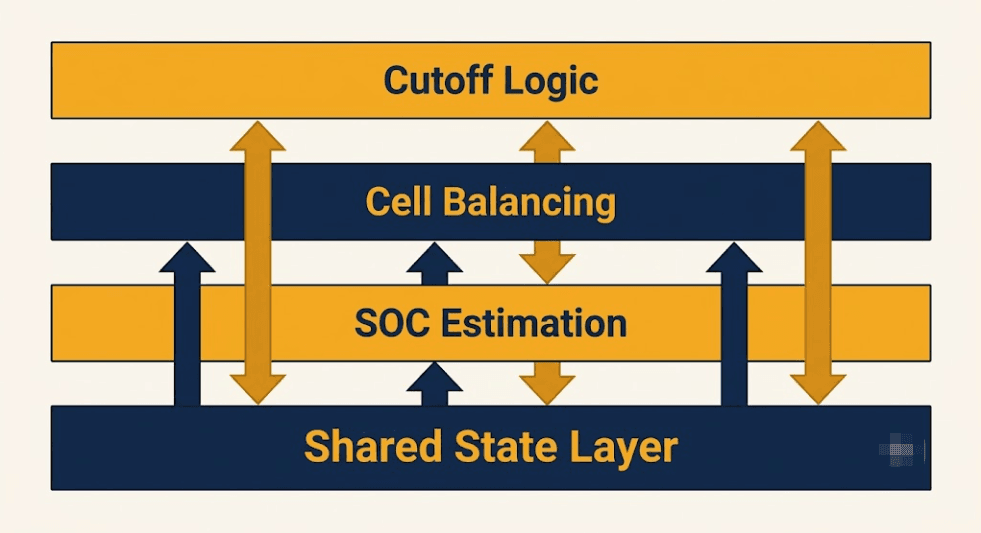
Three failure modes show up again and again in LFP BESS operation. SOC readings drift from reality. Cells pull apart from each other in service. Cutoffs trip before the pack is actually empty. Most teams treat SOC drift and cell imbalance and premature cutoffs as three separate bugs. They are not. All three trace back to one root cause: LFP’s flat voltage curve. This guide covers SOC drift and cell imbalance and premature cutoffs as one connected design problem, not three separate ones, and shows where to fix each layer.
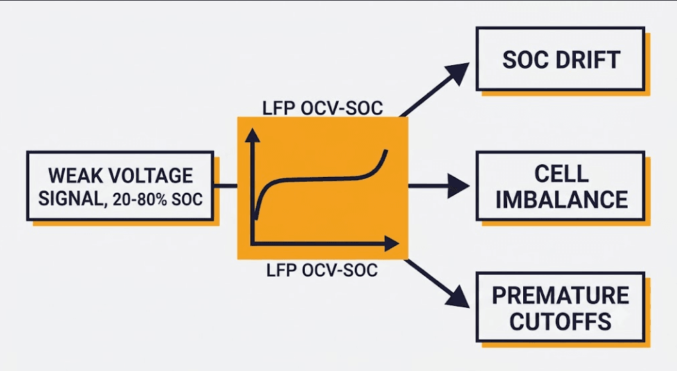
⚡ Quick Answer SOC drift and cell imbalance and premature cutoffs in an LFP BESS all stem from the same root cause. LFP’s flat OCV-SOC curve gives weak voltage signal across most of the operating range. Fixing this needs a matched design at three layers: SOC estimation (the model), cell balancing (the pack), and cutoff logic (the trip point). All three should share one live state, instead of running as separate modules.
Why LFP’s Flat Voltage Curve Drives SOC Drift and Cell Imbalance
LFP cells sit near 3.2–3.3V across roughly 80% of their usable range. A cell at 30% SOC looks almost identical to a cell at 70% SOC on voltage alone. This flat region is the reason SOC drift and cell imbalance and premature cutoffs all show up together in the same systems.
Weak voltage signal means SOC estimation has little to correct against. As a result, it drifts unless the model is built carefully. Weak voltage signal also means cell-to-cell differences hide longer before anyone notices. A pack can drift out of balance for weeks before the voltage spread becomes visible. Furthermore, a weak voltage signal means a cutoff tuned only to a fixed trip voltage cannot tell resistance-driven sag from real depletion. It trips early, stranding capacity the cell still has.
None of these three problems is really about SOC, balancing, or cutoffs on their own. SOC drift and cell imbalance and premature cutoffs are all downstream of the same flat curve. That is why fixing them one at a time, in isolation, tends to under-deliver.
Designing the SOC Estimation Layer for SOC Drift and Cell Imbalance
The estimation layer needs a model, not just a lookup table. LFP’s flat curve makes simple OCV lookup unreliable during operation. Coulomb counting works but drifts without a reset point, and that drift compounds with cycling. An Extended Kalman Filter, built from an equivalent circuit model fitted to HPPC test data, corrects itself continuously against tiny voltage signals that other methods miss.
Getting this layer right matters beyond the SOC number itself. A biased estimate feeds false signals into the other two layers, discussed below. Our EKF SOC estimation design guide covers the model-building and covariance-tuning steps in full.
Mitigating In-Service Cell Imbalance and SOC Drift
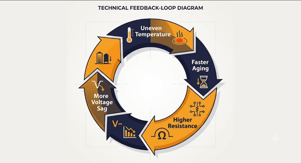
Cell imbalance is not just a factory-matching problem. Even a well-matched pack drifts apart over years, driven mainly by uneven heat. A cell running a few degrees hotter ages faster, gains resistance faster, and sags more under load — which can push it hotter still. Left unmanaged, that feedback loop turns a small temperature gap into a real capacity gap.
Design against this at two levels: thermal layout, sized around worst-case gradients rather than pack averages, and balancing topology matched to the cycling profile. Light daily cycling tolerates passive balancing. Heavy cycling or a persistent thermal gradient needs active balancing to keep pace. Our in-service cell imbalance guide covers both levers in depth.
Designing a Dynamic, DCIR-Adaptive Cutoff
A fixed cutoff voltage assumes fresh-cell resistance at room temperature. Real packs age and get cold. Their internal resistance rises on both counts, sagging more under identical load, which trips a static cutoff earlier and earlier even though real capacity remains.
A DCIR-adaptive cutoff fixes this by calculating the trip voltage in real time. It uses measured current and a resistance value pulled from an HPPC-derived lookup table, indexed by SOC, temperature, and cell age. This alone recovers up to 10% of effective throughput in mid-to-late project life that a static cutoff would otherwise strand. Our DCIR-adaptive cutoff design guide covers the full lookup-table structure.
Closing the Loop: Sharing State Across All Three
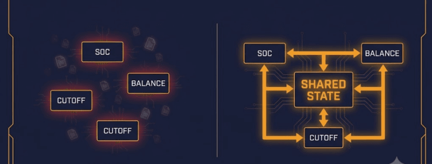
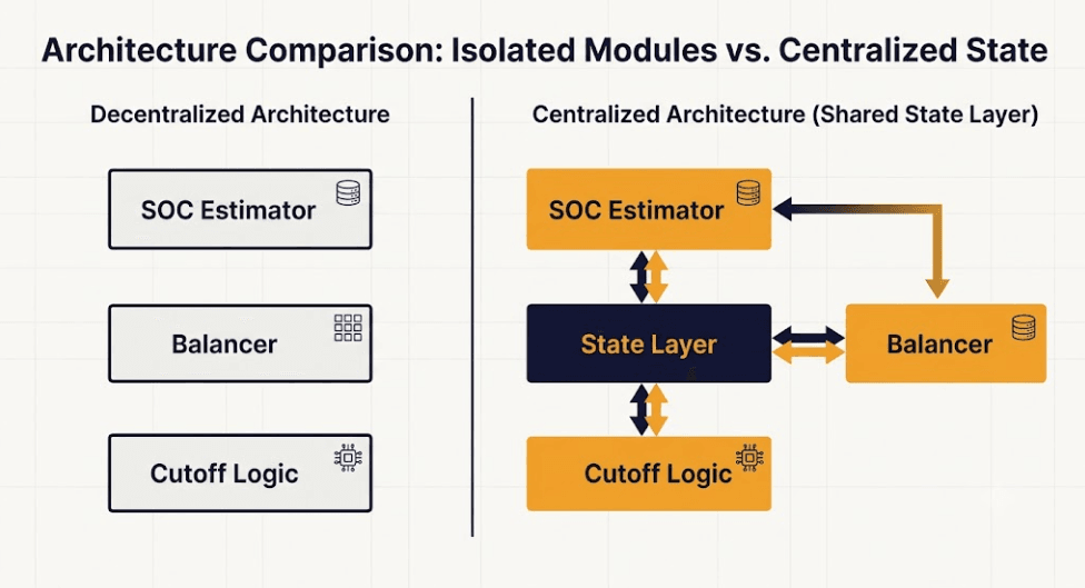
Building these three layers correctly in isolation still leaves a gap. This is where SOC drift and cell imbalance and premature cutoffs stop being separate design problems and start needing one shared answer. Each layer can run its own internal estimate of pack state, and small timing differences let those estimates quietly disagree. The estimator’s SOC value, the balancer’s voltage-spread reading, and the cutoff logic’s resistance calculation should all reference the same live data, not three separate copies of it.
This shared-state design also creates a natural place to catch developing faults. A cell whose resistance departs sharply from its neighbors is worth flagging. This matters most when that departure doesn’t track the pack’s overall aging trend. It’s a signal that’s much harder to catch when each subsystem only sees its own narrow slice of the picture. Our integrated BMS control architecture guide covers how to build that shared layer without a full BMS redesign.
How This Differs From a Buyer’s Checklist
This guide is a design reference, not a procurement checklist. If you’re evaluating a supplier’s BMS rather than architecting one, our BMS for LiFePO4 batteries guide covers the specs and questions to ask before you buy. If your problem sits further upstream — sorting and matching cells before a pack is even assembled — see our cell matching before pack assembly guide. This guide picks up once the pack is designed and in service, addressing SOC drift and cell imbalance and premature cutoffs as they actually show up over years of operation.
This same coordination challenge shows up in the research too. A study on distributed Kalman filtering across battery pack cells explores this tradeoff for thermal estimation specifically, finding that distributed approaches can track a centralized estimate closely when properly designed — the same coordination problem this guide addresses for SOC, balancing, and cutoff logic. Get that coordination wrong, and the failure mode this guide’s shared-state approach is built to avoid shows up instead.
Key Takeaways
SOC drift and cell imbalance and premature cutoffs are not three unrelated bugs — they are one shared-root-cause design problem. All three trace back to LFP’s flat OCV-SOC curve, which gives weak voltage signal across most of the operating range. Fix the estimation layer with a properly parameterized and tuned EKF, not a raw lookup table. Imbalance gets fixed at the thermal-layout and balancing-topology level, not just at factory cell matching. Cutoffs need a DCIR-adaptive design that accounts for real-world resistance, not a fixed datasheet value. Then close the loop: share state across all three layers so they reinforce each other instead of quietly disagreeing.
Frequently Asked Questions
Are SOC drift, cell imbalance, and premature cutoffs really connected problems?
Yes. All three trace back to LFP’s flat voltage curve, between roughly 20% and 80% SOC. That curve gives weak signal for SOC estimation. It hides cell-to-cell differences longer. It keeps a fixed cutoff from telling resistance sag apart from real depletion.
Do I need to fix all three layers at once?
Not necessarily in one project phase, but design them with the same shared-state architecture in mind from the start. Retrofitting shared state after each layer was built in isolation is more work than designing it in from the beginning.
How is this different from a standard BMS buyer’s guide?
A buyer’s guide covers what specs and questions to check before purchasing a BMS. This guide covers how to design or tune those systems once you own the architecture — the estimation model, the balancing strategy, and the cutoff logic itself.
Most BMS designs treat SOC estimation, cell balancing, and cutoff protection as three separate modules. Each one runs its own logic. Each one reads its own inputs. This works, but it leaves value on the table. An integrated BMS control architecture ties these three functions together instead. They share one live state, not three separate guesses. This guide covers what that shared state looks like, and why it matters for LFP. New to BMS fundamentals first? Our BMS explained guide covers the basics before returning here.
⚡ Quick Answer An integrated BMS control architecture means the SOC estimator, the cell balancer, and the cutoff logic all read from one shared, current view of each cell’s voltage, resistance, and temperature. Without this link, each subsystem can act on a slightly different picture of the pack, and small disagreements between them compound into real errors.
Why Three Separate Modules Create Hidden Errors
This challenge is related to a broader question in battery-pack monitoring: whether separately-run, local estimators can be trusted to agree with a fully centralized view. Research on distributed Kalman filtering across battery pack cells explores this tradeoff for thermal estimation specifically, finding that distributed approaches can track a centralized estimate closely when properly designed — the same coordination problem this article addresses for SOC, balancing, and cutoff logic. A BMS built as three separate modules seems simpler at first. But each module often keeps its own internal estimate of pack state. The estimator has its own SOC value. The balancer has its own view of cell voltage spread. The cutoff logic has its own read on present resistance. These three views should agree. In practice, small timing gaps and separate filtering choices let them drift apart, even by a small amount.
A Concrete Example of the Problem
Picture a cell under a sudden high-current pulse. The estimator’s filter may lag the true voltage sag. The lag can run a few hundred milliseconds. The cutoff logic reads raw current and voltage directly. So it reacts faster. It might trip a cutoff. The estimator’s own SOC value says this should not happen yet. Without shared state, this looks like a bug. An integrated BMS control architecture fixes it. Both systems read the same current-corrected voltage, in real time. The mismatch does not occur.
What Shared State Means for an Integrated BMS Control Architecture
An integrated BMS control architecture is not one giant algorithm. It is a shared data layer that each function reads from and writes to. At minimum, this layer holds present cell voltage, present current, present temperature, the estimator’s current SOC output, and the present DCIR value drawn from the resistance lookup table. Every subsystem calculates from this same set of numbers, on the same update cycle.
Update Timing Matters as Much as the Data Itself
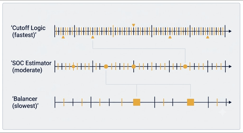
Sharing the right data at the wrong update rate still causes disagreement. The cutoff logic needs the fastest update path. A hard voltage limit can be reached in milliseconds, under a current spike. The SOC estimator can run on a slower cycle instead. Its correction task is inherently smoother. Design the shared state layer so each subsystem pulls at its own needed rate. Do not force one single rate onto all three.
How Subsystems Interact in an Integrated BMS Control Architecture
With shared state in place, the three subsystems can do more than avoid disagreement. They can actively support one another. The estimator’s SOC output can flag the balancer toward cells worth watching. The balancer’s voltage-spread data can flag the estimator when a cell’s behavior looks abnormal, rather than just imbalanced. The cutoff logic’s live DCIR reading, drawn from the same lookup table an EKF SOC estimation design pulls its resistance model from, keeps both systems working from one resistance picture instead of two.
Flagging Faults Instead of Silently Adapting
A well-built integrated BMS control architecture also creates a natural place to catch faults. If the shared DCIR reading from one cell departs sharply from its neighbors, and that departure does not track with the pack’s overall temperature or aging trend, the architecture can flag it as a possible fault, tied to the same in-service cell imbalance and DCIR drift patterns covered elsewhere in this series. This is far harder to catch when each subsystem only sees its own narrow slice of the picture.
Implementing an Integrated BMS Control Architecture Without a Full Redesign
For how centralized, modular, and wireless BMS topologies differ in where this shared layer can physically live, see our BMS architecture guide. Building an integrated BMS control architecture does not usually require new sensors. Most BMS hardware already measures voltage, current, and temperature at a resolution that supports this. The work is mostly in firmware: defining the shared data structure, setting update rates per subsystem, and routing each function’s calculation through the shared layer instead of an isolated local copy.
A Practical Migration Path
Start with the two subsystems most likely to disagree today: the SOC estimator and the cutoff logic, since both read current and voltage directly and both act on threshold logic. Confirm they draw from one shared, current-corrected voltage value before adding the balancer into the same layer. This staged approach limits the scope of any one firmware change and makes each step easier to validate on its own.
Key Takeaways
Three separate BMS modules can quietly disagree, even when each one works correctly on its own. An integrated BMS control architecture fixes this with one shared data layer for voltage, current, temperature, SOC, and DCIR, read by all three subsystems. Update timing matters as much as the shared data itself; each subsystem should pull at the rate its own task needs. Shared state also creates a natural place to flag developing faults, since a real fault shows up as one cell’s data breaking pattern against the rest of the shared picture.
Frequently Asked Questions
Does an integrated BMS control architecture need new hardware?
Usually not. Most BMS hardware already measures voltage, current, and temperature at a fine enough resolution. The work is mainly firmware: building a shared data layer and routing each subsystem’s calculation through it.
Which two subsystems should be integrated first?
Start with the SOC estimator and the cutoff logic. Both read current and voltage directly, and mismatches between them are the most likely to show up as a false or late cutoff trip.
How does an integrated BMS control architecture help catch developing faults?
When every subsystem shares one live view of each cell, a real fault shows up as that cell’s data breaking pattern against its neighbors and against the pack’s overall trend, rather than being missed by a subsystem that only sees its own narrow slice of the picture.
Cell matching before pack assembly sets a good starting point. But it does not stay good forever. In-service cell imbalance builds up over years. It builds long after the pack leaves the factory well matched. Heat, aging, and cycling all pull cells apart again. This guide covers the design choices that slow that drift. It covers thermal layout, balancing topology, and how imbalance control ties back into SOC estimation.
⚡ Quick Answer In-service cell imbalance grows mainly from two sources after assembly: uneven pack temperature, and the uneven aging that follows from it. Good thermal design and the right balancing topology both slow this drift. Neither one fixes a pack that started out badly matched.
Why In-Service Cell Imbalance Differs from Factory Mismatch
Factory cell matching solves the starting-point problem. Our cell matching before pack assembly guide covers that stage in depth. It groups cells by voltage, capacity, and resistance before assembly. In-service cell imbalance is a different, ongoing problem, however, because even a well-matched pack drifts apart over time. The BMS balances small gaps every cycle. But the size of that gap depends on design choices made outside the BMS itself.
The Feedback Loop Between Heat and Aging
This pattern matches published research on thermal gradients in lithium-ion packs, which found that uneven internal temperature drives inhomogeneous degradation and resistance growth well before a pack reaches end of life on paper. Heat is the main driver of in-service cell imbalance. A cell that runs hotter than its neighbors ages faster. It loses capacity faster and, as a result, it gains resistance faster too. Consequently, that resistance rise makes it sag more under load. More sag can make it run hotter still, at the same current. This is a feedback loop. Left unmanaged, a small temperature gap can grow into a real capacity gap. This can happen within a few years of daily cycling.
Designing Thermal Layout to Limit Imbalance
Thermal design is the first lever against in-service cell imbalance. It acts before the BMS ever needs to balance anything. For the specific causes of uneven pack temperature — coolant path position, cell position within the rack, and current-path resistance — and the ΔT targets a well-designed system should hit, see our cell temperature gradients guide. The takeaway for imbalance control specifically: any gradient beyond those targets does not just cost efficiency. It feeds directly into the heat-aging-resistance loop above, and the wider the gradient, the faster the affected cells pull away from the rest of the pack.
Design Around the Worst Case, Not the Average
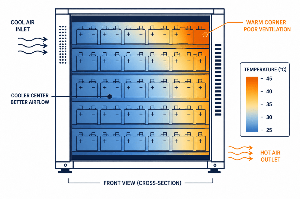
A common mistake sizes cooling around the pack’s average temperature. Average temperature can look fine. Meanwhile, individual cells can sit well outside it. Measure the worst-case gradient across the pack instead of the mean. Design cooling around that number. This resistance rise is the same mechanism covered in our cell internal resistance guide. A pack running meaningfully above those ΔT targets — commonly the case in a poorly ventilated rack corner — is exactly the failure mode that accelerates in-service cell imbalance in the affected cells, over a multi-year service life.
Choosing a Balancing Topology for the Cycling Profile
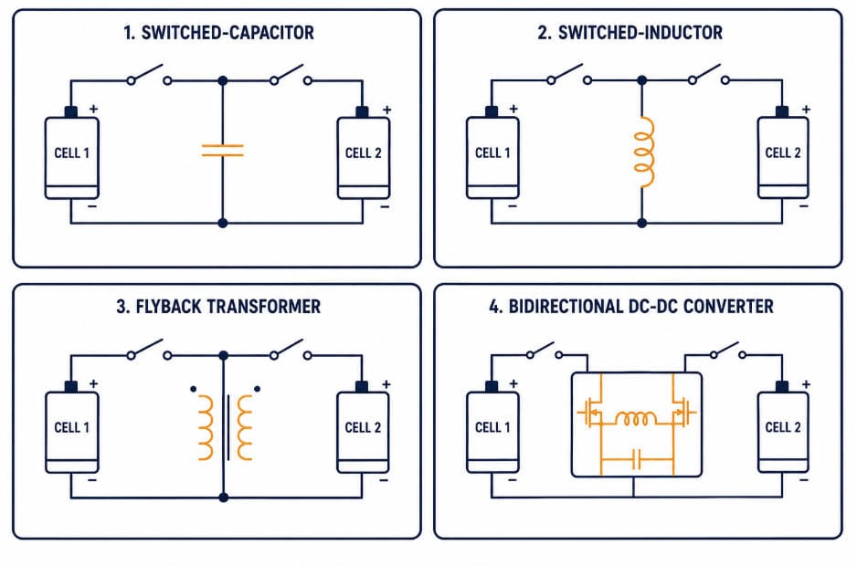
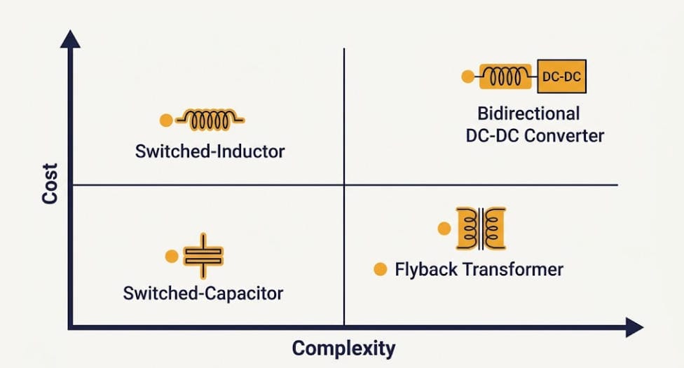
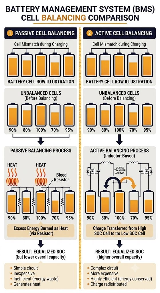
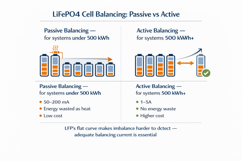
Balancing topology is the second lever. Passive balancing bleeds excess energy off higher-SOC cells as heat. It is simple and low-cost. It works fine for light daily cycling with well-matched cells. But passive current is small. It is often just tens to a few hundred milliamps. It cannot keep pace with fast-building imbalance under heavy cycling or a strong thermal gradient.
Feature
Passive Balancing
Active Balancing
Typical current
Tens to a few hundred mA
1–5A
Cost
Low
Higher, more hardware
Best fit
Light daily cycling, well-matched cells
Heavy cycling, thermal gradients, long-duration assets
Energy handling
Bleeds excess as heat
Moves energy between cells
Effect on in-service cell imbalance
Slows drift on light-use systems
Keeps pace with faster-building drift
When Active Balancing Earns Its Cost Against In-Service Cell Imbalance
Active balancing moves energy between cells instead of burning it off. It corrects gaps far faster, at one to several amps. This higher cost pays off in three cases. First, systems that cycle more than once daily, since imbalance gets less rest time between corrections. Second, systems with a thermal gradient that design alone cannot remove — the same resistance growth this drives also affects cutoff timing; see our DCIR-adaptive cutoff guide. Third, long-duration systems built for fifteen years or more, where small ongoing gains add up to real lifetime value.
Linking Imbalance Back to SOC Estimation
In-service cell imbalance and SOC estimation accuracy feed each other. A design that treats them as separate problems will underperform. A biased SOC estimate can send the balancer a false signal. It might correct a gap that is not really there. Or it might miss one that is. This is the same shared-state problem seen in EKF SOC estimation design. The balancer and the estimator both need one current, shared view of each cell. They should not run on two readings that can quietly disagree.
Setting a Practical Alert Threshold
A voltage spread over 50 to 100 millivolts across cells is a common alert threshold on LFP. The chemistry’s flat curve means even a real SOC gap may show only a small voltage difference. Log these events instead of reacting to one reading. A single high-current moment can cause a spread that resolves on its own.
Key Takeaways
In-service cell imbalance differs from factory cell matching. It is driven mainly by heat, and the aging that heat speeds up. Thermal layout is the first line of defense, especially sizing cooling around worst-case gradients, not pack averages. Balancing topology should match the cycling profile. Passive balancing suits light daily cycling. Active balancing earns its cost in heavy-cycling, high-gradient, or long-duration systems. Imbalance control and SOC estimation should share state, not run as separate systems, since each one affects the accuracy of the other.
Frequently Asked Questions
What causes in-service cell imbalance if the pack started well matched?
Uneven pack temperature is the main driver. Hotter cells age faster and gain resistance faster. That raises sag under load, which can push the cell hotter still. The gap compounds over years of cycling.
Does active balancing fix a pack that started out mismatched?
No. Active balancing corrects ongoing in-service cell imbalance much faster than passive balancing. But neither approach can create capacity a weak cell never had. A bad starting mismatch still needs fixing at the cell-matching stage, before assembly.
What voltage spread signals a real in-service cell imbalance problem on LFP?
A spread over 50 to 100 millivolts is a common threshold worth checking. Still, the trend across cycles matters more than any single reading.
⚡ Quick Answer: What Is Cell Matching? Cell matching is the process of sorting battery cells by voltage, capacity, and internal resistance before they go into a pack, so cells with similar characteristics end up grouped together. It happens on the factory floor, before assembly. This is not the same thing as BMS balancing, which corrects drift after the pack is already built and in use. Skipping cell matching does not make a pack unsafe by itself, since the BMS still protects it. However, it does mean the BMS has to work much harder from day one. As a result, the pack’s real-world capacity and cycle life will likely fall short of what the cell datasheet promises.
1. Why Cell Matching Happens Before the BMS Gets Involved
Cell matching is a manufacturing step that happens before a single cell ever reaches a pack. Even cells from the same production batch are not identical. Small differences in electrode coating thickness, electrolyte fill, and formation cycling leave every cell slightly different. Capacity, voltage, and internal resistance all vary a little, even when the datasheet lists one number for all of them. In a single cell, this variation does not matter. Once dozens or hundreds of cells connect into a pack, though, it matters a great deal.
The BMS will eventually correct some of this drift through balancing, as covered in our complete battery management system guide. Cell matching, however, happens earlier. It is a manufacturing step, not a BMS function, and it exists to reduce how much correction the BMS has to do later.
2. Three Criteria Used to Sort Cells: Voltage, Capacity, and Resistance
Cell matching typically screens for three characteristics. Each one affects the pack differently. As a result, a thorough process checks all three rather than relying on just one.
Voltage (or SOC) matching — technicians group cells by their resting voltage after a defined charge or discharge point. This is the simplest check to run. It also catches the most obvious mismatches quickly.
Capacity matching — technicians charge and discharge test each cell to measure actual usable Ah, then group cells with similar capacity together. This matters most for series strings, since the lowest-capacity cell sets the ceiling for the whole string.
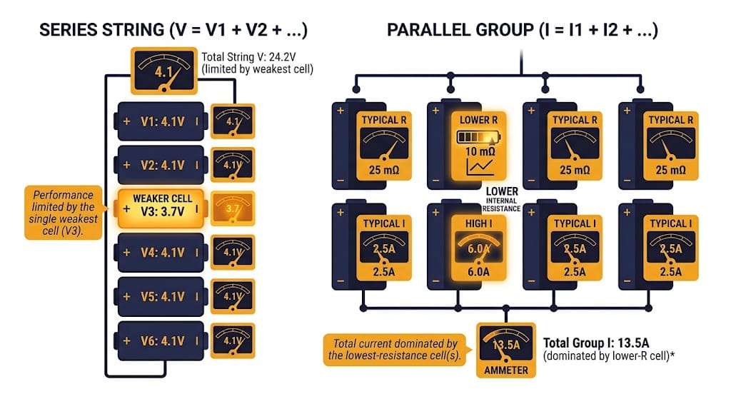
Internal resistance matching — technicians measure resistance using one of two methods, DCIR or ACIR, then group similar-resistance cells into the same parallel group. This matters most for parallel groups, since a lower-resistance cell otherwise takes more than its fair share of current.
High-volume manufacturers often combine all three, and internal resistance testing itself splits into two distinct methods worth understanding.
DCIR vs ACIR: Two Ways to Measure Internal Resistance
DCIR (DC internal resistance) testing applies a current pulse to the cell and measures the resulting voltage drop. Technicians then calculate resistance directly from Ohm’s law. This method closely reflects how the cell behaves under a real load, since it uses an actual current step rather than a small signal. The tradeoff is speed: each pulse needs time to apply and settle, which slows down high-volume sorting.
ACIR (AC internal resistance) testing instead applies a small alternating current signal, commonly at 1 kHz, and reads the resulting impedance directly. This method runs much faster than DCIR, which is why many production sorting lines use it as a first-pass screen. However, ACIR mostly captures the cell’s high-frequency ohmic resistance. It does not fully capture the slower electrochemical charge-transfer resistance that DCIR testing reveals.
In practice, many manufacturers use ACIR for fast first-pass screening across an entire incoming batch, then apply DCIR pulse testing to verify cells before they go into the same series string or parallel group. A supplier who only mentions one of these two methods is likely doing the faster, less thorough version alone.
3. Series Strings vs Parallel Groups: Different Priorities
Series and parallel connections fail differently when cells are mismatched. For this reason, they need different matching priorities.
In a series string, cells share the same current, but their voltages differ based on individual state. The weakest cell — the one with the lowest capacity — reaches its low-voltage cutoff first during discharge. Likewise, it hits its high-voltage cutoff first during charge. As a result, that one weak cell limits the usable capacity of the entire string. This happens even though the other cells still have energy left. This is why capacity matching matters most for series strings.
In a parallel group, cells share the same voltage, but current splits between them based on internal resistance. A cell with lower resistance pulls more current than its neighbors. In turn, it works harder and ages faster. Over time, that uneven current sharing can widen the resistance gap further, creating a feedback loop. Left unchecked, this loop drives localized accelerated aging in the same cells, cycle after cycle. That localized wear is what leads to premature pack failure, well before the rest of the pack reaches end of life. For a buyer, that translates directly into a shorter calendar life and a worse return than the datasheet cycle life implied. This is why resistance matching matters most for parallel groups.
☀️ Resistance matching matters most for parallel groups. 💡 The Thermal Feedback Loop: Internal resistance mismatch and localized heating reinforce one another. For a deeper look at how temperature imbalances accelerate this degradation, read our guide on Cell Temperature Gradients in BESS
4. What Happens If You Skip Cell Matching
Skipping cell matching does not make a pack dangerous on its own. A properly designed BMS still enforces voltage and temperature limits, regardless of how well matched the cells are. What changes, instead, is how hard the BMS has to work, and how much capacity the pack actually delivers.
If cells arrive at noticeably different SOC and go into a pack without matching, the BMS must run a large initial balancing pass. This happens the first time the pack charges. Passive balancing currents are typically small — often just tens to a few hundred milliamps — compared to the pack’s full Ah rating. Correcting a large initial mismatch this way can take many hours. In some cases, it takes several charge cycles before the pack reaches a properly balanced state.
Beyond the slow start, an unmatched pack often never fully closes the gap. If capacity variation between cells is large enough, ongoing balancing keeps the weakest cell from falling further behind. Still, balancing cannot manufacture capacity that a weak cell simply does not have. The pack’s usable capacity, therefore, ends up set by its weakest link, cycle after cycle.
5. Top-Balance vs Bottom-Balance: Which Comes First
When manufacturers match cells by connecting them in parallel before final assembly, the SOC point at which this happens changes the outcome.
Bottom-balance matching connects cells in parallel at a low SOC, often close to how they arrive from the manufacturer. This approach is simple and fast. However, it only aligns the cells at the bottom of the charge curve. The pack will likely still need a top-of-charge balancing pass once assembled and charged for the first time.
Top-balance matching, instead, charges the parallel-connected cells to a high SOC before final assembly, typically near the top of the charge curve. This produces a better-aligned pack from the first charge. That is because the region where mismatch matters most for safety and full capacity gets addressed early. The tradeoff is time: bringing a large batch of cells to a matched high-SOC state takes more equipment and more hours before assembly can begin.
6. Cell Matching at Scale: How Manufacturers Grade Cells for Utility BESS
At utility scale, matching thousands of cells by hand is not practical. Instead, high-volume manufacturers run automated sorting lines. These measure voltage, capacity, and resistance for every incoming cell. Grading software then groups cells into matched sets before they ever reach the assembly line.
For a BESS buyer, this raises a practical question worth asking directly: does the supplier grade and match cells before assembly, or does the pack rely entirely on the BMS to fix mismatch after the fact? Independent testing resources such as Battery University document just how differently DCIR and ACIR readings can diverge on the same cell, which is exactly why asking a supplier which method they use, and at which stage, is worth doing directly.
A supplier who can show incoming cell test data is doing meaningfully more quality control than one who simply points to their BMS’s balancing feature. Look, in particular, for a specific matching tolerance — for example, a defined percentage spread in capacity, or a defined milliohm band in resistance.
7. Questions to Ask Your Cell or Pack Supplier
Do you test and match cells by voltage, capacity, and internal resistance before assembly, or only one of these?
For internal resistance, do you use DCIR, ACIR, or both — and at which stage does each method apply?
What matching tolerance do you use? For example, what percentage spread in capacity, or what milliohm band in resistance?
Do you keep incoming cell test data on file? Can you provide it for the specific batch used in our order?
For series strings, how do you decide which cells go together — capacity, resistance, or both? Our BMS algorithms guide covers how the BMS itself later measures DCIR for SOH estimation, which is a useful comparison point when you ask this question.
Is matching done at a low SOC, a high SOC, or both, before final assembly?
Conclusion: Matching Sets the Ceiling the BMS Can’t Raise
A BMS is very good at correcting small, ongoing drift between cells. It is not designed, however, to compensate for a pack that started out badly mismatched. Cell matching before pack assembly sets the baseline the BMS then has to maintain for the life of the system. A well-matched pack lets the BMS do its normal job: fine-tuning small differences over time. A poorly matched pack, by contrast, forces the BMS into a losing battle against a gap it cannot close, cycle after cycle.
When evaluating a cell or pack supplier, ask specifically how they match cells before assembly, including whether they use DCIR, ACIR, or both. Do not just ask how the BMS balances them afterward. For supplier evaluation more broadly, see our BESS supplier BMS evaluation guide. The cell matching answer says a lot about how much real capacity and cycle life you can expect to see in practice.
☀️ Need Help Evaluating a Cell Matching Process? Sunlith Energy reviews incoming cell test data, matching tolerances, and pack assembly quality control for BESS projects from 50 kWh upward. Contact us before you finalize a cell or pack supplier.
Frequently Asked Questions About Cell Matching
Is cell matching the same as BMS balancing?
No. Cell matching happens before assembly. It is a manufacturing step that sorts cells by voltage, capacity, and internal resistance, so similar cells end up grouped together. BMS balancing, on the other hand, happens after assembly, correcting the small drift that develops during normal use. Matching reduces how much balancing the BMS has to do; it does not replace it.
What is the difference between DCIR and ACIR matching?
DCIR testing applies a current pulse and calculates resistance from the voltage drop using Ohm’s law, closely reflecting real load behavior. ACIR testing applies a small AC signal, commonly at 1 kHz, and reads impedance directly, which runs much faster but mostly captures high-frequency ohmic resistance rather than the full picture. Many manufacturers use ACIR for fast first-pass screening, then confirm with DCIR before final grouping.
What is the difference between capacity-based and resistance-based sorting?
Capacity-based sorting groups cells with similar usable Ah, and matters most for series strings, since the lowest-capacity cell sets the ceiling for the whole string. Resistance-based sorting, by contrast, groups cells with similar internal resistance, and matters most for parallel groups, since a lower-resistance cell will otherwise pull more than its fair share of current.
Does skipping this step make a battery pack unsafe?
Not directly. A properly designed BMS still enforces voltage and temperature limits, no matter how well the cells were matched. That said, skipping this step does mean the BMS must run a larger initial balancing pass. In turn, the pack’s real-world capacity may fall short of the datasheet value, since the weakest cell limits the whole pack.
Should I ask my BESS supplier for this test data?
Yes. Ask whether the supplier tests and matches cells by voltage, capacity, and internal resistance before assembly, and which resistance method they use. A supplier who can provide incoming cell test data for your specific batch is demonstrating a real quality control process, not just relying on the BMS to compensate after the fact.
Is top-balance or bottom-balance better?
Top-balance, which aligns cells at a high SOC before assembly, generally produces a better-aligned pack from the first charge. That is because it addresses the top-of-charge region where mismatch matters most. Bottom-balance is faster, but the pack will likely still need a top-of-charge balancing pass once assembled.
⚡ Quick Answer: What Are BMS Algorithms? BMS algorithms go far beyond SOC estimation. A production BMS runs several algorithms at once: SOH estimation, SoP, SoE, cell balancing logic, contactor sequencing, isolation monitoring, safety diagnostics, and RUL prediction. For BESS, the quality of these BMS algorithms decides dispatch reliability, warranty defensibility, and second-life value — not just SOC accuracy.
1. Beyond SOC: The Full BMS Algorithm Stack
Most talk about BMS algorithms stops at State of Charge. SOC matters. But it is only one output from a stack of six or more BMS algorithms running at once.
For a deeper dive into OCV lookup, Coulomb counting, and Extended Kalman Filter SOC methods, see our dedicated guide: BMS SOC Estimation Methods Explained. This article picks up where those leave off, covering the advanced firmware algorithms that drive aging, dispatch limits, safety, and long-term asset value.
A BESS operator or EPC should understand what each BMS algorithm actually calculates. Marketing language often overstates what firmware really runs. The sections below walk through each algorithm layer in build order: health first, then power and energy limits, then balancing, then safety, then long-term prediction.
2. SOH Algorithms: How BMS Algorithms Track Battery Aging
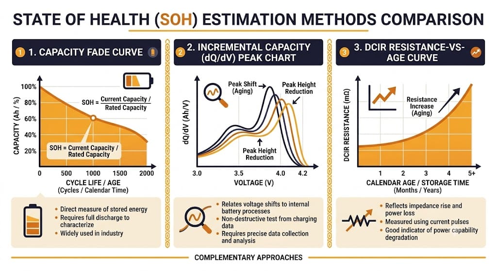
State of Health (SOH) is the second most important number a BMS produces after SOC. It is also far harder to calculate correctly. SOH shows how much usable capacity and performance remain compared to a new cell. A cell rated at 100 Ah that now delivers 92 Ah has an SOH of roughly 92%.
Unlike SOC, SOH cannot reset with one charge cycle. The BMS must infer it from long-term trends. This makes SOH-focused BMS algorithms fundamentally different from SOC algorithms.
Capacity Fade Tracking Algorithm
The simplest SOH algorithm compares measured full-charge capacity against rated nameplate capacity. The BMS records the Ah delivered between two known SOC points, typically 100% to 0%. It then compares that figure against the original rated capacity.
This method is accurate but slow. It produces one new SOH data point per full cycle. Many BESS installations rarely complete a true 100–0% cycle. Partial-cycle capacity fade algorithms estimate the fade rate from partial cycles instead, using coulomb-counted throughput and known depth-of-discharge. These partial-cycle BMS algorithms carry more uncertainty than full-cycle measurements.
Incremental Capacity Analysis (ICA) Algorithm
Incremental capacity analysis is a more advanced SOH algorithm. It examines the shape of the voltage curve, not just its endpoints. As a cell ages, specific peaks in its incremental capacity curve (dQ/dV) shift and shrink. Each shift pattern correlates with a specific degradation mechanism: lithium plating, active material loss, or electrolyte decomposition. ICA-based BMS algorithms can tell different aging causes apart, not just report one percentage. For the electrochemistry behind why lithium plating happens in the first place — and how it interacts with the slower SEI layer growth every LFP cell experiences — see our guide on SEI layer growth and lithium plating in LFP cells.
ICA-based BMS algorithms can tell different aging causes apart, not just report one percentage. This matters for warranty claims and second-life valuation. A cell degrading from normal calendar aging is a very different asset than one degrading from a manufacturing defect or thermal abuse event.
The tradeoff is cost. ICA needs high-resolution voltage sampling during specific charge segments. Not every BMS platform captures this data by default.
DCIR-Based SOH Algorithm
DC internal resistance (DCIR) rises as a cell ages, mostly independent of capacity fade. A DCIR-based SOH algorithm applies a known current pulse and measures the resulting voltage drop. It then calculates internal resistance using Ohm’s law, and compares that value against a baseline resistance-versus-age curve for the specific cell model.
DCIR-based SOH algorithms run faster than capacity-fade methods, since a short current pulse is enough — no full cycle required. This makes them useful for spotting outlier cells early, often before capacity fade becomes visible.
The limitation is temperature sensitivity. DCIR shifts a lot with cell temperature. An accurate DCIR-based BMS algorithm must correct every reading against a resistance-versus-temperature-versus-age model calibrated for the exact cell in use.
SOH Algorithm Comparison
Method
What It Measures
Update Frequency
Best For
Capacity fade tracking
Ah delivered vs. rated capacity
Once per full cycle
Systems with regular full cycles
Incremental capacity analysis (ICA)
dQ/dV curve shape and peak shift
Per qualifying charge segment
Distinguishing aging mechanisms, warranty claims
DCIR-based SOH
Internal resistance rise vs. baseline
Per current pulse (fast)
Early outlier-cell detection, partial-cycle systems
Most premium BMS platforms combine all three algorithms: DCIR for fast, frequent checks; capacity fade tracking as the long-term anchor; and ICA for diagnostic deep-dives when a cell shows early warning signs.
3. SoP Algorithm: What BMS Algorithms Tell the Inverter
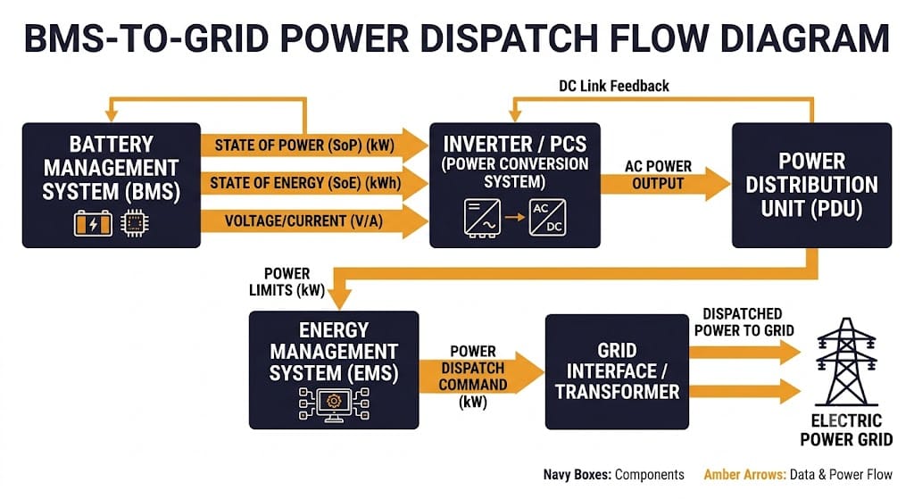
State of Power answers a different question than SOC or SOH. It asks not “how much energy is stored,” but “how much power can this pack safely deliver or accept right now.” The SoP algorithm calculates the maximum charge and discharge power available for a set time window, typically 1, 10, or 30 seconds. It weighs current SOC, temperature, cell voltage limits, and internal resistance.
This number goes straight to the inverter or PCS and to the energy management system (EMS). Without an accurate SoP algorithm, the EMS either under-dispatches or over-dispatches. Under-dispatching leaves revenue on the table during a frequency regulation or peak-shaving event. Over-dispatching triggers a protection cutoff mid-event, which is worse for grid-service contract compliance.
SoP gets harder to calculate at temperature and SOC extremes. A pack at 10% SOC or −5°C has much lower discharge SoP than the same pack at 50% SOC and 25°C, even with similar energy content. A well-designed SoP algorithm accounts for voltage sag under load. It does not rely on static cell voltage limits alone, and it uses the same internal resistance data the SOH algorithm tracks.
4. SoE Algorithm: Usable kWh, Not Just Percentage
SOC gives you a percentage. The SoE algorithm gives you the actual usable kilowatt-hours remaining. It factors in current SOH, temperature derating, and the depth-of-discharge limits set for the system. Two BESS units showing 60% SOC can have very different SoE if one has degraded to 85% SOH and the other sits near 98% SOH.
For asset owners running dispatch contracts or virtual power plant participation, SoE is the number that actually sets revenue capacity. A BMS that only reports SOC forces the EMS to apply a separate correction factor for aging, and that workaround adds error. A BMS with a proper SoE algorithm reports usable energy directly, already corrected for real-world capacity.
5. SoR and SoF Algorithms: Diagnostic and Dispatch-Readiness Checks
Two less-discussed BMS algorithms round out the state-estimation stack.
State of Resistance (SoR) tracks internal resistance as its own diagnostic metric, separate from its role as a SOH input. Rising resistance in a single string or module is often the earliest sign of an emerging fault. It can flag a loose busbar connection or accelerated local aging before it shows up in the pack-level SOH number.
State of Function (SoF) is a composite go/no-go algorithm. It combines SOC, SOH, SoP, temperature, and active fault flags into one dispatch-readiness signal. The EMS checks this signal before committing the BESS to a grid-service event. A pack can have fine SOC and SOH individually and still fail SoF — for example, if a temperature sensor reads near its fault threshold. SoF exists to stop the EMS from dispatching a unit that has energy on paper but should not be trusted for that event.
6. Cell Balancing Algorithms: Passive vs Active Control Logic
Cell balancing keeps every cell in a series string at a matched voltage and SOC. The control logic behind it is itself a BMS algorithm worth understanding, not just a hardware feature.
This balancing logic is especially vital—and complex—when dealing with the flat voltage plateaus of LFP chemistry; for a deeper look at hardware and balancing nuances there, read our specific guide on BMS for LiFePO4 batteries.
Passive Balancing Algorithm Logic
A passive balancing algorithm finds the highest-voltage cell in a string during charge. It then switches a bleed resistor across that cell, burning off excess energy as heat until the cell matches the pack average. The control logic usually triggers balancing only above a voltage or SOC threshold, commonly near the top of charge, where cell mismatch matters most for safety and full-charge capacity.
Design choices matter more than the hardware here. A poorly tuned threshold balances too aggressively, wasting energy and building unnecessary heat. Too conservative a threshold lets mismatch build up for many cycles.
Active Balancing Algorithm Logic
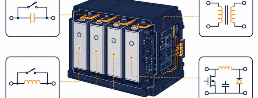
An active balancing algorithm moves charge from higher-voltage cells to lower-voltage cells, using inductors, capacitors, or switched-capacitor networks. It does not just burn off the difference as heat. The control logic is more complex: it must sequence several transfer paths at once, avoid oscillation between cells close in voltage, and decide when further balancing no longer justifies the switching losses.
For grid-scale BESS with thousands of series-parallel cells, the balancing algorithm’s efficiency affects round-trip efficiency and effective cycle life directly. A well-balanced pack ages its weakest cells more slowly, since those cells spend less time at voltage extremes.
7. Contactor and Isolation BMS Algorithms
Two safety-critical BMS algorithms operate below the level most BMS content ever discusses. They matter a great deal for BESS commissioning and daily operation.
Pre-Charge Sequencing Algorithm
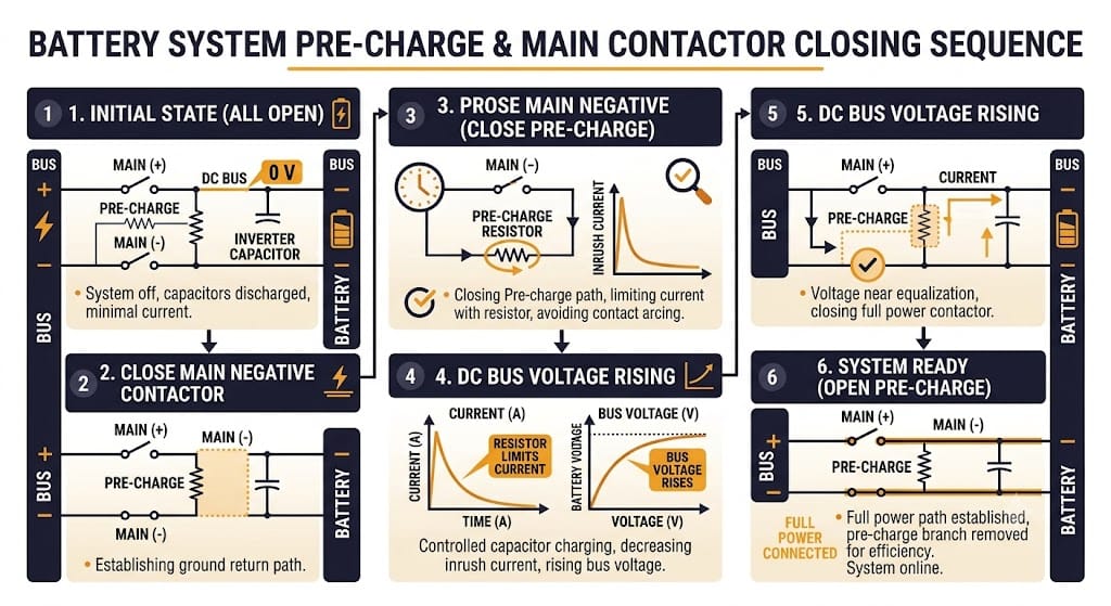
When a BESS connects to its inverter or DC bus, a large voltage gap between the battery and a discharged bus can spike current high enough to weld contactor contacts or blow fuses. The pre-charge sequencing algorithm closes a smaller pre-charge contactor through a current-limiting resistor first. It watches the bus voltage rise toward battery voltage, and only closes the main contactor once the gap falls within a safe threshold, typically a few percent.
The algorithm must also set a timeout and a fault response. If bus voltage fails to rise as expected in time, that signals a downstream fault. A well-designed sequence aborts the connection instead of forcing the main contactor closed anyway.
Isolation Monitoring Algorithm
High-voltage BESS strings must stay electrically isolated from chassis ground. The isolation monitoring algorithm injects a small test signal, or measures leakage current, between the HV bus and chassis ground. It then calculates an isolation resistance value. A common safety threshold is 500 ohms per volt of system voltage — a 750V BESS string needs at least 375,000 ohms of isolation resistance under this rule.
A slowly degrading isolation reading, even one still above the fault threshold, is an early warning worth flagging. It usually points to moisture ingress, insulation wear, or a developing ground fault well before it trips a hard fault.
8. Safety Diagnostic Algorithms: MAVD, RdV, and Early Fault Detection
Beyond voltage, current, and temperature thresholds, advanced BMS platforms run pattern-based diagnostic algorithms. These catch failure modes before they reach a hard safety limit.
Maximum Allowable Voltage Deviation (MAVD) algorithms compare each cell’s voltage against the pack average in real time. A cell drifting outside its expected deviation band can signal an internal short, a connection fault, or local degradation — even while it stays within absolute safe voltage limits. Because MAVD looks at relative deviation, not absolute thresholds, it often catches faults earlier than simple over-voltage or under-voltage protection.
Resistance-derivative or rate-of-change (RdV) algorithms track how fast a cell’s voltage or resistance is changing, not just its current value. A cell with rapidly climbing resistance is a different risk than one with stable but elevated resistance, even if both report the same SOH today. RdV algorithms flag the rate of change itself as its own alarm condition.
These diagnostic layers matter most for large-format BESS, where a single degrading cell among thousands can go unnoticed until it causes a string-level fault. Standards bodies such as the IEC publish safety requirements for stationary lithium battery systems that reference exactly this kind of deviation monitoring.
Furthermore, if you are deploying assets in the European market, these algorithmic diagnostics are critical for compliance; see our EU batteries regulation EU 2023 1542 complete guide for a full breakdown of the data and safety mandates.
Ask suppliers whether their BMS runs deviation and rate-of-change diagnostics on top of standard threshold protections — this is a real differentiator between a basic BMS and a genuinely safety-engineered one.
9. RUL Prediction Algorithms and Second-Life Value
Remaining Useful Life algorithms take SOH trend data and project forward. They estimate how many more cycles or years remain before the pack falls below an end-of-life threshold, commonly 70–80% of original capacity.
Three RUL Algorithm Approaches
Empirical RUL algorithms fit a degradation curve — often exponential, or a two-stage linear-then-accelerating shape — to historical SOH data for the specific chemistry and use profile. They then extrapolate forward. These are cheap to run and reasonably accurate for well-studied LiFePO4 chemistries with large datasets for a quick way to model these degradation curves yourself based on cycle depth and temperature, you can check out our interactive battery cycle life calculator. But they assume future use resembles the past.
Physics-based (electrochemical) RUL algorithms simulate the degradation mechanisms directly: lithium plating, SEI growth, active material loss. They predict RUL from first principles. These are more accurate under changing use conditions, but they need detailed cell-level parameters that cell suppliers do not always share.
Machine-learning RUL algorithms train on large fleets of historical degradation data. They predict RUL from current sensor patterns without an explicit physical or empirical formula. These can beat both other approaches when trained on a large enough fleet of the same cell type and use case. But they need a lot of historical data, and they can behave unpredictably outside the conditions they trained on.
Why RUL Algorithm Accuracy Matters for BESS Economics
RUL accuracy affects two commercial decisions directly: warranty reserve calculations for suppliers, and second-life asset valuation for owners. A BESS pack projected to hold 80% capacity for ten more years is worth much more on the second-life market than one with an uncertain or steeply declining RUL curve. Lower-demand second-life uses, like residential backup or slow-cycling grid support, depend on that projection being credible.
For utility-scale BESS operators planning eventual asset disposition, ask your BMS or EMS supplier which RUL modeling approach they use, and what fleet data backs it. Battery aging research from national labs such as NLR (National Laboratory of the Rockies) increasingly informs these models. Ask whether RUL confidence intervals are reported alongside the point estimate — a single RUL number with no range is hard to use for financial planning.
10. Questions to Ask Your BMS Supplier About Algorithms
Marketing language often claims “advanced algorithms” without saying which ones actually run in firmware. For a structured framework on auditing these capabilities during procurement, see our guide on BESS supplier BMS evaluation.
The following targeted questions will help you separate real algorithmic depth from a basic protection-only BMS with technical-sounding labels:
Which SOH algorithm does the BMS use — capacity fade tracking, ICA, DCIR-based, or a combination? A BMS that only runs capacity fade tracking will be slow to catch outlier cells in systems that rarely complete full cycles.
Does the BMS calculate SoP and SoE algorithms, or only SOC and SOH? Without SoP output, the EMS must apply conservative blanket power limits, which lowers dispatch revenue.
What isolation resistance threshold does the algorithm enforce, and how is it temperature- and time-compensated? A static threshold with no trend monitoring misses slow isolation decay.
Does the balancing algorithm run passive, active, or both, and what triggers a balancing cycle? Ask for the specific voltage or SOC threshold, not just “the BMS balances cells.”
What RUL algorithm approach is used, and is a confidence interval reported? A point-estimate RUL number with no uncertainty bounds has limited use for financial and warranty planning.
Conclusion: Algorithm Depth Is the Real BMS Differentiator
SOC estimation gets most of the attention in BMS marketing. But the BMS algorithms that actually protect a BESS investment over its 10–20 year life sit one layer deeper. SOH tracking catches aging mechanisms early. SoP and SoE outputs maximize safe dispatch revenue. Balancing logic gets tuned for the specific pack architecture. Safety diagnostics catch deviation before it becomes a fault. RUL models come with defensible confidence intervals.
When you evaluate a BMS or a BESS supplier, ask specifically which of these BMS algorithms are implemented, and how they were validated. Do not settle for “the BMS monitors SOC and SOH.” The answer reveals whether you are buying genuine algorithmic engineering or a basic protection circuit with confident marketing copy.
☀️ Need a BMS Algorithm Review for Your BESS Project? Sunlith Energy reviews BMS algorithm implementations — SOH methodology, SoP/SoE accuracy, balancing logic, and RUL modeling — for BESS projects from 50 kWh upward. Contact us before you commit to a supplier.
Frequently Asked Questions About BMS Algorithms
What algorithms does a BMS run besides SOC estimation?
A production BMS runs several algorithms beyond SOC: SOH estimation (capacity fade tracking, incremental capacity analysis, or DCIR-based methods), SoP and SoE calculations, cell balancing control logic, contactor pre-charge sequencing, isolation monitoring, safety diagnostics such as voltage-deviation and resistance-rate-of-change monitoring, and often RUL prediction models.
What is the difference between the SOH and SoP algorithms in a BMS?
The SOH algorithm measures how much capacity and performance a battery has lost compared to new, shown as a percentage. The SoP algorithm measures how much power the battery can safely deliver or accept right now, based on current SOC, temperature, and internal resistance. SOH looks backward at cumulative aging. SoP looks at the immediate power ceiling for dispatch decisions.
Why does the SoP algorithm matter for BESS dispatch even if SOC looks fine?
A pack can show good SOC while still having a low SoP at cold temperatures or high internal resistance. That means it cannot deliver the power a grid-service event needs without tripping a voltage protection limit. An EMS that only checks SOC before dispatch risks committing to an event the pack cannot actually support.
How does the DCIR-based SOH algorithm work?
The BMS applies a known current pulse and measures the resulting voltage drop. It calculates internal resistance using Ohm’s law, then compares that resistance against a temperature-compensated baseline curve for the specific cell model. This algorithm runs faster than capacity-fade tracking, since it needs no full charge-discharge cycle.
What is a good RUL algorithm confidence level for a utility-scale BESS?
There is no single universal number — it depends on the modeling approach and available fleet data. What matters more is whether the supplier reports a confidence interval at all, rather than a single point estimate, and whether the model has been checked against real fleet degradation data for the same cell chemistry and use profile.
Do I need an active balancing algorithm for a grid-scale BESS, or is passive enough?
Passive balancing works fine for many commercial and lower-cycling systems. For utility-scale BESS with high cycling frequency and large series strings, an active balancing algorithm usually improves round-trip efficiency and cuts accelerated aging in weaker cells. That can justify its added cost over the system’s lifetime.
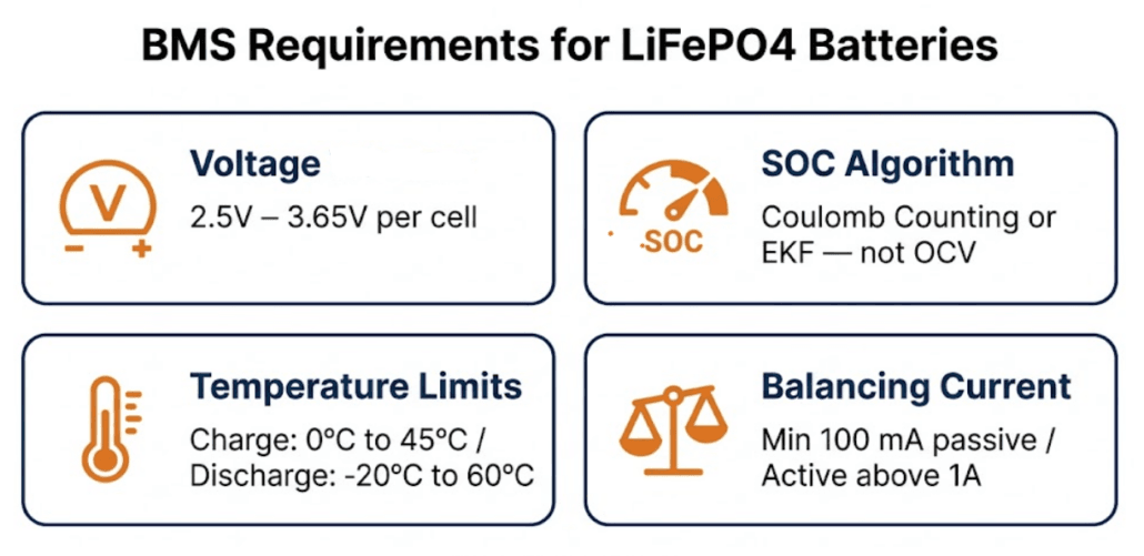
⚡ Quick Answer: What Does a BMS for LiFePO4 Need? A BMS for LiFePO4 batteries must enforce a cell voltage window of 2.5V–3.65V, use Coulomb counting or Kalman filtering for accurate SOC (not OCV alone), provide at least 80–100 mA balancing current for passive systems, monitor temperature at multiple points, and halt charging below 0°C. These requirements differ significantly from NMC — a BMS designed for NMC will underperform on LFP cells.
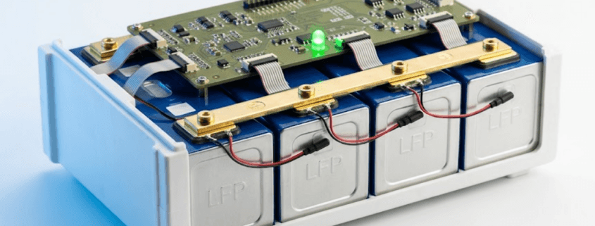
LiFePO4 (LFP) is the dominant chemistry for solar storage, commercial BESS, and off-grid systems. Its long cycle life, thermal stability, and safety advantages make it the first choice for most stationary applications. However, LFP also has specific characteristics that place unique demands on the BMS for LiFePO4.
Not every BMS is built with LFP in mind. Many suppliers use a generic platform across multiple chemistries. Consequently, an NMC-designed BMS on LFP cells shows poor SOC accuracy and slow balancing. It also lacks the specific protections LFP needs.
This guide covers the key requirements for a BMS for LiFePO4 — voltage parameters, SOC methods, balancing current, and temperature limits. It also includes the supplier questions that reveal whether a BMS is genuinely built for LFP.
New to battery management systems? Read our complete BMS explainer guide first, then return here for the LFP-specific detail.
1. Why LiFePO4 Places Unique Demands on the BMS
LFP’s chemistry gives it three properties that directly shape what the BMS must do. Understanding these properties is the starting point for evaluating any BMS for LiFePO4.
The Flat Voltage Curve: LiFePO4’s Biggest BMS Challenge
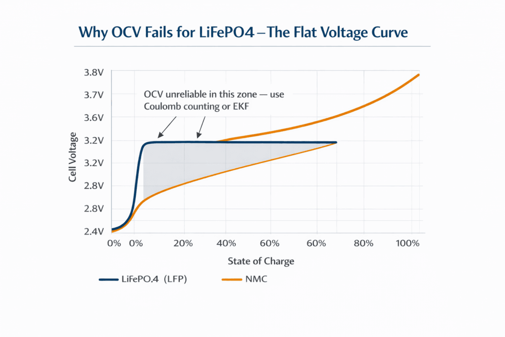
LFP cells operate near 3.2V–3.3V across most of their usable SOC range. Specifically, from 20% to 80% SOC, the voltage barely moves. This is unlike NMC, where voltage drops steadily and predictably as the cell discharges.
Consequently, the BMS cannot rely on voltage alone to estimate SOC. A cell at 50% SOC and a cell at 30% SOC look almost identical on voltage. As a result, any BMS that uses OCV as its primary SOC method will be wildly inaccurate on LFP during operation.
This is the most important LFP-specific BMS requirement. A wrong SOC estimate causes early shutdowns and surprise overcharge events. It also wastes usable energy by setting overly cautious capacity limits.
Chemical Stability: LiFePO4 Still Needs BMS Protection
LFP’s iron-phosphate cathode is chemically very stable. Its thermal runaway threshold is 270°C–300°C — far higher than NMC’s 150°C–210°C. This stability means the BMS has more time to respond to developing faults. However, it does not mean LFP needs less protection.
Over-discharge below 2.5V per cell damages the anode permanently. Overcharge above 3.65V per cell damages the cathode. Both need fast BMS action. The stability advantage of LFP reduces thermal risk — but it does not reduce voltage protection needs.
Wide Operating Temperature Range
LFP handles temperature extremes better than NMC. It operates from -20°C to 60°C on discharge and from 0°C to 45°C on charge. However, charging below 0°C causes lithium plating. This is a permanent form of anode damage that accumulates with each cold-temperature charge cycle.
The BMS must, therefore, actively halt charging when cell temperature drops below 0°C. This is a hard protection requirement, not a soft warning. For more on how temperature affects LFP lifespan, see our guide on temperature impact on LiFePO4 cycle life.
2. LiFePO4 BMS Voltage Parameters: The Exact Numbers
Voltage parameters are the foundation of any BMS for LiFePO4 configuration. These values define the safe operating window for each cell. The BMS enforces them through contactor control and charge/discharge current limiting.
Parameter
LFP Value
What Happens If Breached
Nominal cell voltage
3.2V
Reference point for system design — not a limit
Charge cutoff (max)
3.65V per cell
Permanent cathode damage above this — BMS must disconnect
Discharge cutoff (min)
2.5V per cell
Permanent anode damage below this — BMS must disconnect
Recommended operating range
2.8V–3.4V per cell
Staying within this range extends cycle life significantly
Cell voltage balance tolerance
±20mV typical
Wider spread indicates balancing failure or weak cell
Low voltage pre-warning
2.7V–2.8V
BMS should alert before hard cutoff — allows graceful shutdown
Why Cell-Level Monitoring Is Non-Negotiable
These voltage limits apply to individual cells — not to the overall pack voltage. In a 16S LFP pack (16 cells in series), the nominal pack voltage is 51.2V. However, one weak cell can hit its 2.5V discharge cutoff while the pack voltage still reads 49V — well above the apparent safe threshold.
A BMS that monitors only pack voltage will therefore miss this event entirely. The weak cell gets driven below its safe limit and suffers permanent damage. Consequently, cell-level individual voltage monitoring is the most basic non-negotiable requirement for any BMS for LiFePO4.
Voltage Tolerance in the BMS Hardware
The accuracy of the voltage measurement circuit matters. For LFP, a measurement tolerance of ±5–10mV per cell is acceptable. Some premium BMS platforms achieve ±1–2mV. Tighter tolerances mean the BMS can set closer operating limits and extract more usable capacity from the pack.
Ask your supplier: what is the cell voltage measurement accuracy of the BMS? If they cannot answer, that is a red flag.
3. SOC Estimation for LiFePO4: Why OCV Alone Fails
LFP’s flat voltage curve makes OCV-based SOC estimation unreliable — the BMS must use Coulomb counting or Kalman filtering instead
SOC estimation is where most generic platforms fail. It is, therefore, the most important technical question to ask any BMS for LiFePO4 supplier.
Why OCV Fails for LFP
OCV lookup works by mapping a resting cell voltage to a SOC value. It uses a table built from cell tests. This works well for NMC because NMC voltage drops steadily as the cell discharges.
LFP, however, produces an almost flat voltage curve between 20% and 80% SOC — roughly 3.2V to 3.3V across this entire range. As a result, a cell at 25% SOC and a cell at 75% SOC look nearly identical on OCV. The BMS cannot distinguish between them. Consequently, an OCV-based BMS on LFP shows SOC readings that jump erratically and fail to track the actual charge state.
OCV is only useful for LFP after the battery has rested for at least 30–60 minutes with no current flowing. It is, therefore, a valid method for setting the initial SOC estimate at startup — not for real-time tracking.
Coulomb Counting: The Minimum Standard for LFP
Coulomb counting integrates current over time to track charge entering and leaving the battery. It is the most widely used SOC method in real-time operation. It is also the minimum acceptable standard for any BMS for LiFePO4.
Coulomb counting is accurate over short periods. However, it drifts over time. Sensor errors, temperature effects, and small unmeasured currents all add up. Without regular recalibration, the SOC estimate can drift by 2–5% over several days.
Best practice: The BMS should recalibrate SOC to 100% when the battery reaches full charge voltage (3.65V per cell) and to 0% when it reaches the discharge cutoff (2.5V per cell). These are reliable anchor points that correct accumulated drift automatically.
Extended Kalman Filter: The Gold Standard for LFP
The Extended Kalman Filter (EKF) is the most accurate SOC method for LFP. It combines Coulomb counting with a cell behaviour model. Continuously, it corrects the estimate by comparing the model’s output to the actual measured voltage.
EKF handles LFP’s flat curve far better than OCV. It does not rely on voltage to estimate SOC. Instead, it uses a dynamic model that accounts for temperature, aging, and load history. Furthermore, premium BMS platforms from Texas Instruments, Analog Devices, and Orion BMS use EKF or adaptive Kalman filter variants.
The trade-off is complexity. EKF requires a well-characterised cell model that must be calibrated for the specific LFP cell chemistry in use. A generic EKF implementation calibrated for one cell type will not necessarily be accurate on another. Always ask whether the EKF model was calibrated for the specific cells in your system.
Method
Accuracy on LFP
Key Limitation
Use Case
OCV Lookup
Poor (flat curve)
Useless during operation
Initial SOC at rest only
Coulomb Counting
Good short-term, drifts
Accumulates error over time
Minimum standard — all LFP systems
Coulomb + OCV reset
Good — self-correcting
Needs full charge/discharge cycles
Residential and C&I systems
Extended Kalman Filter
Excellent (±1–2%)
Needs cell-specific calibration
Utility-scale and precision BESS
4. Temperature Requirements for a LiFePO4 BMS
LFP handles temperature better than NMC. However, this does not mean temperature management matters less — it means the safety margins are wider. The BMS must still enforce hard temperature limits and respond to thermal events.
LFP Temperature Operating Limits
Condition
Safe Range
BMS Action Required
Charging temperature
0°C to 45°C
Halt charging below 0°C — lithium plating risk
Discharging temperature
-20°C to 60°C
Reduce current below -10°C; cut off below -20°C
Optimal operating range
15°C to 35°C
No restriction — full rated performance
High temp warning
45°C–55°C
Reduce charge/discharge current; trigger cooling
High temp cutoff
Above 55°C–60°C
Disconnect pack — risk of accelerated degradation
Thermal runaway threshold
~270°C–300°C
Emergency disconnect and alarm — well above normal ops
Temperature Sensor Placement for LFP
The number and placement of temperature sensors directly affects BMS accuracy. For LFP packs, the minimum is one sensor per module. However, in larger systems, multiple sensors per module are standard — at the cell surface, the busbar, and inside the enclosure.
Temperature gradients across a large LFP pack can be significant. A poorly ventilated corner of a battery rack can run 10°C–15°C hotter than the rest. Without adequate sensor coverage, the BMS misses this. Consequently, the hottest cells degrade faster, creating imbalance that shortens the entire pack’s life.
Cold Weather and LFP: The Lithium Plating Risk
Charging LFP below 0°C is one of the most common field mistakes in cold-climate installations. When lithium ions cannot intercalate into the anode at low temperatures, they deposit as metallic lithium on the anode surface instead. This lithium plating is permanent and cumulative.
Specifically, repeated cold-temperature charging causes capacity loss and increases internal resistance. In severe cases, it creates dendrites that cause internal short circuits. The BMS must therefore monitor cell temperature before and during charging. It must halt charge current if any cell falls below 0°C.
5. Cell Balancing Requirements for LiFePO4 BMS
LFP’s flat voltage curve makes cell imbalance harder to detect — the BMS needs adequate balancing current to keep cells in sync
Cell balancing is especially important for LFP. The flat voltage curve makes imbalance harder to spot by voltage alone. Two cells can differ significantly in SOC while showing nearly the same voltage. As a result, the BMS must use current tracking — not just voltage — to detect and correct imbalance.
Minimum Balancing Current for LFP
Passive balancing current determines how quickly the BMS can correct cell imbalance. For LFP systems, the minimum acceptable balancing current depends on system size and cycle frequency.
System Size
Minimum Balancing Current
Why
Residential (under 30 kWh)
50–100 mA
Low cycle frequency — slow balancing keeps up
Small C&I (30–200 kWh)
100–200 mA
Daily cycling creates drift — needs more current to correct
Large C&I (200–500 kWh)
200–500 mA or active
Passive may not keep up — active balancing preferred
Utility-scale (500 kWh+)
Active balancing (1–5A)
Passive is inadequate — active required for long-term performance
When to Specify Active Balancing for LFP
In residential systems with one cycle per day and high-grade A-cell packs, passive balancing at 100 mA is typically sufficient. The cells are well-matched from the factory and, consequently, drift slowly at moderate cycle rates.
Active balancing becomes worthwhile for LFP systems in three situations. First, systems above 500 kWh that cycle daily — imbalance builds faster than passive balancing can fix. Second, systems in variable temperature environments where thermal gradients cause uneven aging. Third, long-duration systems designed for 15+ years where small capacity gains have significant ROI impact.
For a detailed comparison of passive vs active balancing methods, see our complete BMS guide which covers both approaches in depth.
6. Protection Functions: What a LiFePO4 BMS Must Detect
Beyond voltage and temperature, a BMS for LiFePO4 must handle several protection scenarios. Each one has LFP-specific parameters that differ from other chemistries.
Overcharge Protection in a BMS for LiFePO4
The hard overcharge cutoff for LFP is 3.65V per cell. Above this, the cathode undergoes irreversible structural changes. The BMS must therefore disconnect the charge current before any cell reaches this limit. It must do so at the cell level — not the pack level.
Response time should be under 100ms from detection to contactor opening. Additionally, the BMS should implement a pre-warning at around 3.55V–3.60V that reduces charge current (CC-CV charging taper) before the hard cutoff is needed. This protects cells and reduces stress on the contactor.
Over-Discharge Protection for LiFePO4 Cells
The discharge cutoff for LFP is 2.5V per cell. However, the recommended operating minimum is 2.8V — keeping cells above 2.8V significantly extends cycle life. The BMS should therefore implement a two-stage approach: a soft limit at 2.8V that issues a warning and reduces available power, and a hard cutoff at 2.5V that disconnects the pack entirely.
In grid-connected systems, the EMS typically enforces the operational SOC limit well above the hard BMS cutoff. However, the BMS hard limit acts as the last line of defence. It activates if the EMS dispatch fails or if the system enters an unexpected deep discharge scenario.
Short Circuit and Overcurrent Protection
Short circuit response must be in microseconds. The BMS uses a hardware protection circuit — a MOSFET or contactor — that operates independently of the main processor. Software-based response is simply too slow for a hard short circuit event.
Overcurrent protection covers sustained high-current events that are not a hard short. It typically uses a time-delay threshold — for example, 2C discharge for more than 10 seconds triggers a disconnect. The exact settings depend on the cell’s C-rate rating and the load profile.
Cell Voltage Imbalance: A Key LiFePO4 BMS Alert
This is an LFP-specific protection function that many generic BMS platforms handle poorly. LFP cells look similar on voltage even when SOC values differ significantly. As a result, the BMS must monitor cell voltage spread continuously and alert when cells diverge beyond the tolerance threshold.
A spread greater than 50–100 mV across cells indicates a problem. It is typically a sign of a weak cell, a failing balancing circuit, or early degradation. The BMS should log this event and alert the monitoring platform — not simply trigger a hard cutoff.
7. BMS for LiFePO4: Communication and Data Requirements
A BMS for LiFePO4 in a modern BESS must communicate reliably with the inverter, EMS, and monitoring platform. Furthermore, from 2027, EU Battery Passport compliance adds data logging requirements. As a result, communication capability becomes a regulatory issue — not just a technical one.
Communication Protocols: What a BMS for LiFePO4 Must Support
CAN bus 2.0A/B — standard for high-performance and EV-derived BMS platforms; fastest and most reliable
RS485 / Modbus RTU — most common in C&I and utility BESS; compatible with most commercial inverters
CANopen — used in some European industrial applications
MQTT / TCP-IP — required for cloud monitoring and Battery Passport data export
Before specifying a BMS, confirm it works with your inverter’s protocol. A mismatch needs a gateway converter — adding cost, a failure point, and communication lag.
Data Logging Requirements for LiFePO4 BMS Systems
For residential and small commercial LFP systems, minimum data logging should cover SOC, cell voltages, temperatures, cycle count, and fault history. This supports warranty claims and helps diagnose degradation over time.
For systems selling into the EU market after February 2027, the BMS must also log SOH history, energy throughput, and temperature exposure. This data must be in a format compatible with the EU Digital Battery Passport. For full details, see our EU 2023/1542 compliance guide.
8. BMS for LiFePO4 Certifications: What to Check
A BMS for LiFePO4 in a commercial or grid-connected system must hold safety certifications. These confirm the BMS has been tested under fault conditions and meets minimum protection standards.
Standard
Scope
LFP BMS Relevance
UL 1973
Stationary lithium battery systems
Required for US market — covers BMS protection functions
IEC 62619
Li-ion battery safety
International standard — covers voltage, temp, and BMS protection
IEC 62933-5
ESS safety framework
Covers BMS communication, monitoring, and fault response
UN 38.3
Transport safety
BMS must survive vibration and thermal tests for shipping
CE Marking
EU market access
Required for EU sales — covers electrical safety
Always request the full test reports — not just the certificate. A reputable BMS supplier will provide complete documentation without hesitation. If they provide only a certificate image with no underlying test data, treat that as a red flag.
9. How to Evaluate a LiFePO4 BMS: 7 Specific Questions
Generic BMS evaluation questions apply to all lithium chemistries. These seven questions, however, are specifically designed to reveal whether a BMS has been properly configured for LFP cells.
Questions 1–4: Technical Parameters
What SOC algorithm does this BMS use for LFP — and can you show me the accuracy data?
If the answer is OCV lookup, walk away. Ask specifically for SOC accuracy under dynamic load conditions — not just at rest. A good answer is Coulomb counting with OCV reset, or EKF with LFP-calibrated cell model. Ask for the SOC error percentage from their test data.
What is the cell voltage measurement accuracy, and how often does the BMS sample each cell?
For LFP, ±10mV or better is the minimum. Sampling frequency should be at least once per second under normal operation, with faster sampling during charge/discharge transitions. Slower sampling misses brief voltage spikes near the cutoff limits.
Does the BMS halt charging below 0°C at the cell level — not just the ambient temperature?
This is a critical LFP protection requirement. Ambient temperature sensors can give false readings. A cell inside an enclosure can be warmer or colder than the ambient sensor shows. The BMS must therefore use cell-level temperature sensors for this protection. If the supplier uses only one ambient sensor, that is inadequate for LFP.
What is the balancing current, and is it sufficient for the system’s daily cycle rate?
Use the table in Section 5 as your reference. A 50 kWh residential system cycling once daily needs at least 100 mA. A 500 kWh C&I system cycling twice daily needs at minimum 500 mA passive or active balancing. If the supplier cannot tell you the balancing current, that is a red flag.
Questions 5–7: Data and Support
Was the BMS calibrated specifically for the LFP cells in this system — or is it a generic configuration?
SOC accuracy depends on the BMS being calibrated for the specific cell chemistry and capacity. A BMS set up for a 100 Ah CATL cell will not be accurate on a 200 Ah EVE cell. Always ask whether the cell model was calibrated for your specific cells.
What LFP-specific fault codes does the BMS log, and how are they accessible?
Look for: cell voltage imbalance alerts, low-temperature charge inhibit events, SOC drift correction logs, and balancing records. These are essential for diagnosing field problems and supporting warranty claims. A BMS that only logs hard faults — not pre-fault warnings — will miss early signs of cell trouble.
Does the BMS support OTA firmware updates — and is the LFP cell model updatable in the field?
LFP cells change as they age. A BMS with OTA firmware updates can recalibrate its cell model over time. This keeps SOC accuracy high as the cells degrade. It is a premium feature — but it matters a lot for systems designed to last 15+ years.
Conclusion: Match the BMS to the Chemistry
A BMS for LiFePO4 is not the same as a generic lithium BMS. LFP’s flat voltage curve needs a purpose-built SOC method. Its sensitivity to cold charging needs cell-level temperature sensors. Its long cycle life needs strong balancing to keep cells aligned over thousands of cycles.
The seven questions in Section 9 will reveal whether a supplier has genuinely designed their BMS for LiFePO4 — or simply relabelled an NMC platform. The difference matters. Over a 15-year lifespan, a purpose-built BMS for LiFePO4 delivers more usable energy, better SOC accuracy, and fewer field failures.
☀️ Need an LFP BMS Review for Your BESS Project? Sunlith Energy reviews BMS specifications for LFP projects from 50 kWh upward. We check SOC algorithm suitability, voltage parameter configuration, balancing current adequacy, and certification compliance — before you commit to a supplier. Contact us
Frequently Asked Questions
What voltage should a LiFePO4 BMS cut off at?
The hard charge cutoff is 3.65V per cell and the hard discharge cutoff is 2.5V per cell. However, for longer cycle life, the recommended operating range is 2.8V to 3.4V. Operating consistently within this narrower range can significantly extend total cycle count over the system’s lifetime.
Can I use an NMC BMS on LiFePO4 cells?
Technically you can, but the SOC accuracy will be poor. NMC BMS platforms typically use OCV-based SOC, which fails on LFP’s flat voltage curve. The voltage window settings will also be wrong — NMC cells have higher charge cutoffs and different discharge profiles. In practice, an NMC BMS on LFP leads to inaccurate SOC readings, early shutdowns, and reduced usable capacity.
What is the minimum balancing current for a LiFePO4 BMS?
Residential systems under 30 kWh cycling once daily need 50–100 mA passive balancing. Commercial systems above 100 kWh cycling daily need 200 mA or more. Active balancing is preferred for systems above 500 kWh. Low balancing current in a large pack allows imbalance to accumulate — leading to progressive capacity loss.
Does a LiFePO4 BMS need to stop charging in cold weather?
Yes — this is a hard requirement. Charging LFP below 0°C causes lithium plating, which is permanent and cumulative. The BMS must use cell-level temperature sensors to enforce this protection. Ambient sensors alone are not sufficient — cells inside an enclosure can be warmer or colder than the surrounding air suggests.
How accurate should SOC be on a LiFePO4 BMS?
A Coulomb counting BMS with regular OCV resets should achieve ±3–5% SOC accuracy in steady-state operation. An EKF-based BMS with a properly calibrated LFP cell model should achieve ±1–2%. Poor SOC accuracy above ±10% typically indicates OCV-only estimation — or a cell model not calibrated for the specific LFP chemistry.