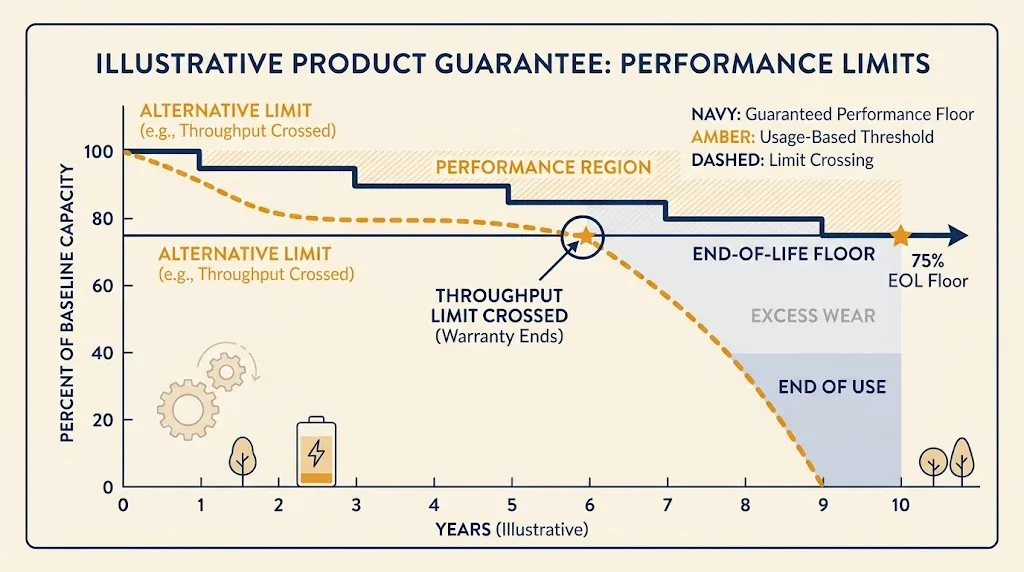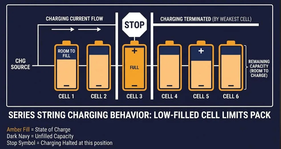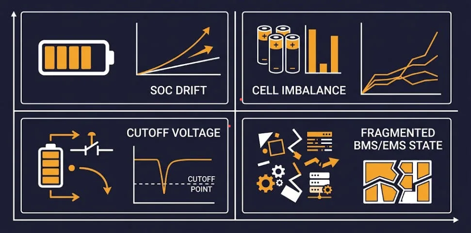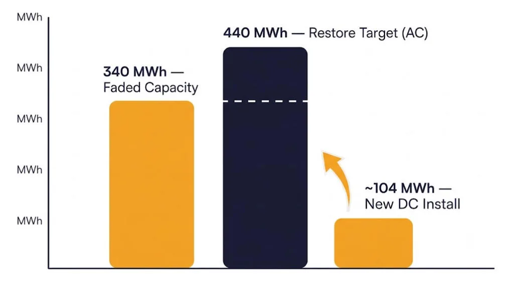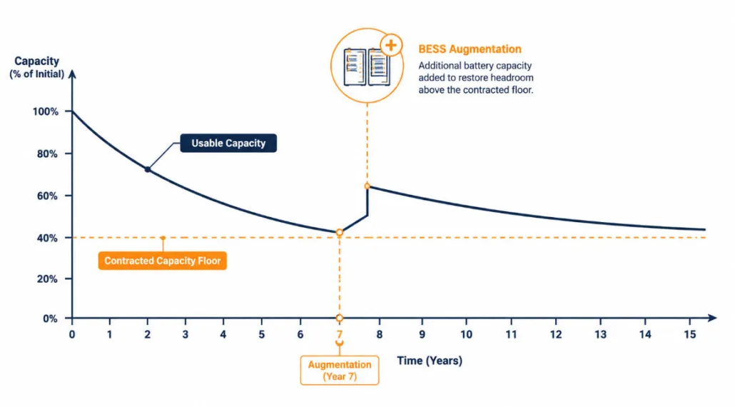
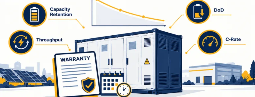
BESS augmentation is the process of adding new battery capacity to an existing energy storage system. It restores or increases capacity lost to degradation. Every BESS loses usable capacity over time. Cycling wears down the cells. Calendar aging adds to it too, even when the system sits idle. So, eventually, the project can no longer deliver the energy or power it promised. BESS augmentation exists to close that gap. It does this by restoring nameplate capacity, or by pushing past it.
Quick Answer BESS augmentation adds new battery capacity to an existing system, later in its life, to restore or increase capacity lost to degradation. It differs from oversizing, which installs extra capacity upfront. Owners execute augmentation one of two ways: AC block addition, which adds a new self-contained power block, or DC shuffling, which reallocates and adds capacity behind the existing inverters.
What Is BESS Augmentation?
BESS augmentation and BESS oversizing solve the same problem. However, they act at different points in a project’s life. Oversizing installs extra capacity on day one. This happens before any degradation occurs. BESS augmentation, on the other hand, adds capacity later. It happens once real-world fade has been measured. Our BESS oversizing guide covers that upfront strategy in full. It also covers the trade-off between the two paths. This guide, instead, focuses on the mid-life path. It covers what triggers augmentation, how it works, and how to plan for it.
BESS Augmentation vs. Oversizing: The Short Version
Neither strategy is strictly better. Oversizing locks in capital and tax credits early. But it carries idle capacity for years. BESS augmentation, in contrast, defers that capital. It depends on good execution years later. By then, battery prices, chemistry options, and site conditions may all have changed.
Factor
BESS Augmentation (Mid-Life)
BESS Oversizing (Upfront)
Capex timing
Deferred to year 5-10
Higher Day-1 cost
Section 48E ITC eligibility
Can face reduced eligibility on added capacity
Full credit on entire capacity at commissioning
Execution risk
Depends on future prices, chemistry, site conditions
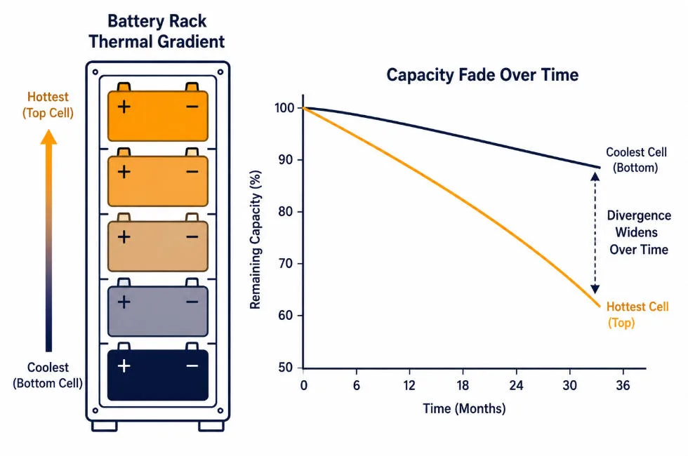
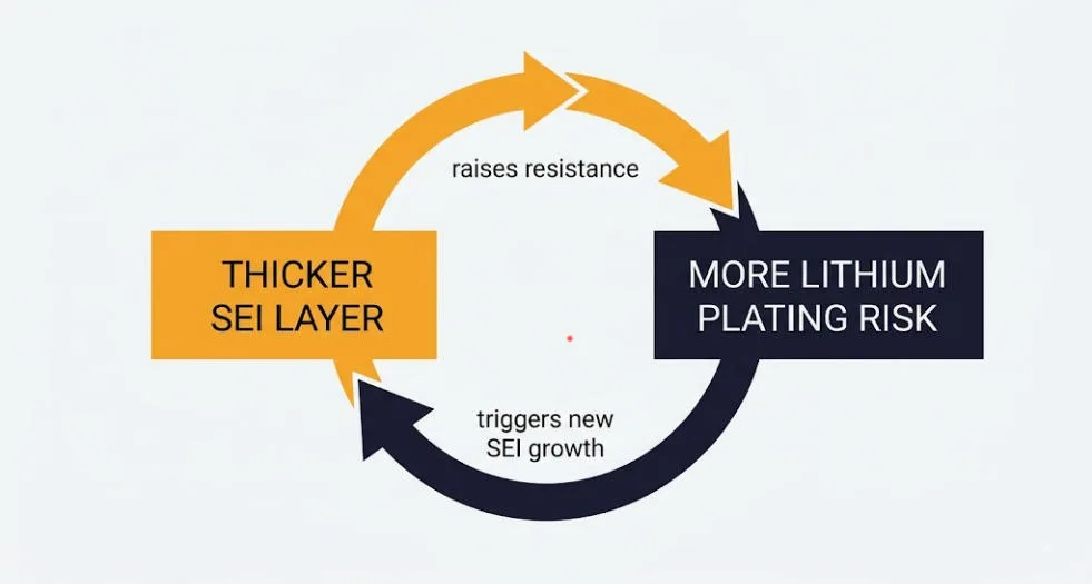
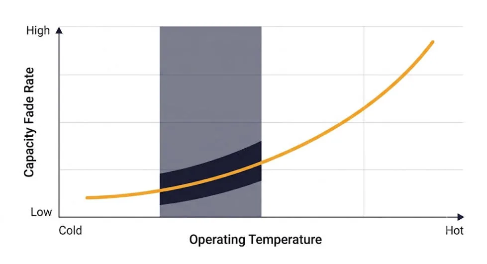
Lithium-ion cells fade with every charge and discharge cycle. Specifically, the protective layer on the anode cracks and reforms with each cycle. This consumes active lithium. High charge rates and cold temperatures also speed up the damage. Meanwhile, calendar time adds a slower fade on top of cycling.
Grid-scale LFP systems commonly lose about 2 to 3 percent of usable capacity per year. As a result, after five to seven years, many projects fall short of their contracted energy or power. That, in turn, threatens revenue directly.
Capacity Guarantees and Tolling Agreements
Most utility-scale BESS projects operate under a tolling agreement or a capacity sale agreement. These contracts are priced against a guaranteed deliverable capacity. This is not simply nameplate capacity at commissioning. So, if degradation erodes that capacity below the contracted floor, trouble follows. The owner then faces liquidated damages or lost revenue. BESS augmentation, therefore, is how owners keep that promise as the asset ages.
These agreements often run 10 to 20 years. So, the augmentation plan is not an afterthought. Instead, it gets built into the financial model at financial close. It sits alongside the degradation curve and the warranty terms.
The Two Paths to BESS Augmentation: AC and DC
There are two ways to physically carry out BESS augmentation. One works on the AC side. The other works on the DC side.
AC Block Addition
First, AC block addition installs a new, self-contained power block next to the existing system. It comes with its own inverters, and often its own transformer too. Because it does not share a DC bus with the old batteries, it avoids voltage and state-of-charge mismatches. It also works with any battery chemistry. As a result, it opens the door to pairing a newer chemistry with an aging LFP fleet.
DC Shuffling
Second, DC shuffling reallocates and adds battery modules behind the inverters already on site. It reuses the existing power conversion equipment. This, in turn, keeps costs down. However, busbar ratings, breaker capacity, and voltage matching all place a ceiling on how much it can add.
For more detail, our AC block addition vs. DC shuffling guide walks through the full technical comparison. It includes a worked example for sizing the restore buffer. It also covers the busbar and short-circuit limits that cap DC shuffling.
What Triggers a BESS Augmentation Decision?
BESS augmentation planning typically starts at a trigger point. That point is when a site’s measured state of health nears the level needed for its contracted output. Operators track this through periodic capacity tests. In addition, battery management system state-of-health estimates support the tracking. So, neither relies on guesswork.
Typical Timing: Year Five to Year Ten
For most grid-scale LFP projects, that point arrives between year five and year ten. Cycling intensity and climate both affect the timing. For instance, hot climates and aggressive cycling schedules push the timeline sooner. On the other hand, shallow cycling, or oversizing at commissioning, pushes it further out.
Planning early matters a great deal. A reactive BESS augmentation project, ordered only after a shortfall occurs, has far less room to negotiate. Because of that, procurement timelines, chemistry options, and price all suffer.
Battery Chemistry and BESS Augmentation Planning
Battery chemistry affects how easily new capacity can be added. LFP has a flat voltage curve. So, it makes voltage matching between old and new modules more forgiving than steeper chemistries like NMC. This is one reason DC shuffling is more common on LFP systems.
AC block addition, however, removes chemistry matching from the equation entirely. The new block runs its own inverters. So, an operator can add a different chemistry, such as sodium-ion, next to an existing LFP fleet. No voltage curves need to line up.
Tax Credits, Costs, and Procurement for BESS Augmentation
The tax picture for BESS augmentation is less favorable than for oversizing. Under Section 48E, the tax credit applies most cleanly to capacity installed at commissioning. Capacity added later, however, can face reduced credit eligibility. It can also add compliance work. This is a core trade-off against upfront oversizing. So, model it carefully before committing to a mid-life augmentation strategy.
Procurement timelines also differ sharply between the two paths. DC shuffling makes no new grid connection. So, it can often skip a fresh interconnection study. AC block addition, in contrast, usually cannot skip that step, since it adds new grid-connected hardware. That difference alone can add months to the schedule.
Cost varies too. DC shuffling generally costs less per megawatt-hour added. This is because it reuses the existing PCS, transformer, and switchgear. AC block addition costs more. However, it buys a clean equipment boundary. It also adds the option to upgrade power conversion technology at the same time.
A Practical BESS Augmentation Planning Checklist
1. Confirm the site’s actual state-of-health trend against the contracted capacity floor.
2. Model the restore buffer in AC terms, then convert it to a DC installation size, accounting for round-trip losses.
3. Choose between AC block addition and DC shuffling based on busbar/breaker headroom, chemistry needs, and permitting timeline.
4. Reserve physical space for future modules if a DC shuffling path is likely.
5. Model the Section 48E tax credit and financing impact of adding capacity mid-life.
6. Build procurement and, if needed, interconnection lead time into the schedule early.
Key Takeaways on BESS Augmentation
1. BESS augmentation restores or increases capacity lost to degradation, later in a project’s life.
2. Most grid-scale LFP projects need to plan for it between year five and year ten.
3. Tolling agreements and capacity sale agreements make augmentation a contractual necessity, not an option.
4. AC block addition and DC shuffling are the two execution paths, with different cost, timeline, and chemistry trade-offs.
5. Augmented capacity can face reduced Section 48E tax credit eligibility compared to capacity installed at commissioning.
Frequently Asked Questions About BESS Augmentation
When Should a Project Plan for BESS Augmentation?
In short, BESS augmentation planning should begin early. It should start as soon as a site’s degradation curve first threatens a future contract obligation. It should not wait until after a shortfall occurs.
What’s the Difference Between BESS Augmentation and BESS Oversizing?
Oversizing installs extra capacity upfront, before degradation happens. BESS augmentation, by contrast, adds capacity later, once real-world fade has been measured. Oversizing generally captures a fuller tax credit. It also carries lower operational complexity. Augmentation, however, defers capital and can benefit from falling battery prices.
Does Augmented Capacity Qualify for the Section 48E Tax Credit?
Capacity installed at commissioning generally qualifies most cleanly for the Section 48E credit. Capacity added later through augmentation, however, can face reduced eligibility or added compliance work. So, this should be modeled carefully before choosing a mid-life strategy.
How Long Does a BESS Augmentation Project Take?
Timelines vary by path. DC shuffling projects typically avoid a new interconnection study. So, they can often move in weeks to a few months. AC block addition projects, on the other hand, usually require new grid-connected hardware. As a result, they more commonly take several months, due to interconnection and permitting steps.
What’s the Difference Between AC Block Addition and DC Shuffling?
AC block addition installs a new, independent power block with its own inverters. It works with any battery chemistry. DC shuffling, in contrast, reallocates and adds capacity behind the existing inverters. It costs less, but it is limited by busbar, breaker, and voltage-matching constraints.
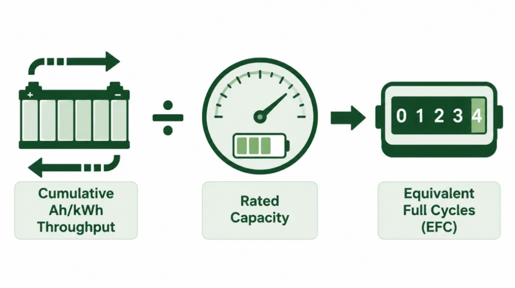
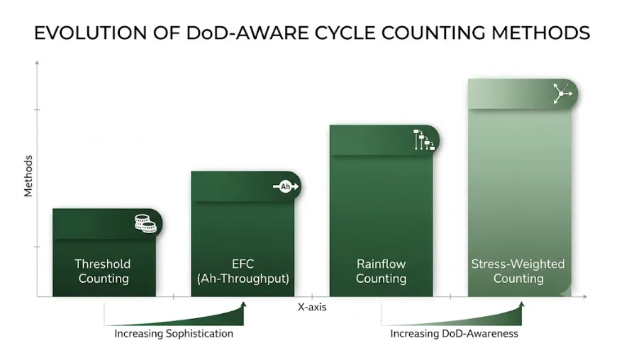
⚡ Quick Answer: What Is BMS Cycle Counting? BMS cycle counting turns raw current and SOC data into a wear metric. First, most systems track Ah/kWh throughput and convert it into Equivalent Full Cycles (EFC). Next, advanced platforms run a rainflow algorithm that splits a messy SOC trace into discrete, depth-weighted cycles. Finally, premium BMS platforms add a stress-weighted layer for C-rate and temperature. As a result, BMS cycle counting feeds SOH and RUL models, not just a simple warranty odometer.
BMS cycle counting sounds simple. In reality, it is one of the least understood functions inside a Battery Management System. Every BESS datasheet shows a number like “6,000 cycles to 80% SOH.” Few buyers ask the obvious follow-up question: how does the BMS actually reach that count in the field? A grid-connected battery rarely swings cleanly from 100% to 0% and back. Instead, it moves up 12%, down 4%, up 20%, down 7%, dozens of times a day. Dispatch signals, solar variability, and frequency-regulation events all drive this pattern. Because of this, converting a noisy trace into one clean cycle number is a genuinely hard firmware problem.
This guide explains exactly how BMS cycle counting works today. First, we cover why simple threshold counting fails for BESS. Next, we break down the rainflow algorithm, borrowed from mechanical fatigue analysis. Then, we show how it solves the partial-cycle problem. Finally, we explain why the datasheet number rarely matches what your BMS reports in the field. For the state-estimation layer this article builds on, see our guides to BMS SOC estimation methods and BMS algorithms explained.
1. Why BMS Cycle Counting Is Harder Than It Sounds
A cycle sounds easy to count: full charge, full discharge, done. However, “one cycle” has no single agreed definition outside the lab. A cell tested for its datasheet rating runs controlled, repeatable 100%–0% swings at a fixed C-rate and temperature. However, a cell inside a grid-connected BESS does nothing of the sort.
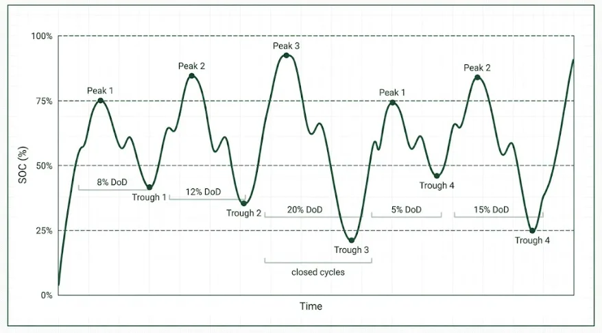
In practice, real-world SOC traces look like a jagged mountain range. Hundreds of small reversals happen every day. A dispatch instruction, a passing cloud, or a short frequency-regulation event can each trigger one. If BMS cycle counting logged every reversal as a cycle, one day of frequency regulation could register thousands of cycles. That would badly overstate wear. On the other hand, a threshold-only method misses just as much. A peak-shaving BESS that stays within the 20–80% band could show almost zero full cycles. Yet it may still have years of hard use behind it.
Neither outcome helps warranty tracking or SOH modelling. For this reason, BMS and EMS firmware rely on purpose-built cycle-counting algorithms instead of simple threshold logic. According to Energy-Storage.News, the industry still lacks one universal definition of a cycle. That gap is exactly why several competing counting methods exist side by side today.
The most basic form of BMS cycle counting sets two SOC thresholds, typically near 95% and 5%. Firmware then adds one to a counter each time the pack completes a full traverse between them. This approach is cheap to build and easy to explain. As a result, it shows up often in low-cost consumer BMS platforms.
For stationary BESS, though, this method falls short. Most BESS installations rarely complete a true top-to-bottom swing. Dispatch strategies deliberately avoid the SOC extremes to protect cycle life (see our guide on the 20/80 rule for batteries). Consequently, a system cycling between 20% and 80% SOC may never trigger a single “full cycle” under this method. That can happen even after years of heavy use. This undercount is precisely why the industry moved toward throughput-based BMS cycle counting instead.
3. Method 2: BMS Cycle Counting With Ah-Throughput (EFC)
This method sits behind almost every commercial BESS warranty. Rather than watching for full swings, the BMS integrates current over time. It uses the same Coulomb-counting math built for SOC estimation. In other words, it adds up every amp-hour that flows in or out of the pack, in either direction. The BMS then divides that cumulative throughput by the pack’s rated capacity. The result is Equivalent Full Cycles, or EFC.
For example, a 500 kWh BESS that has processed 1,000 kWh of cumulative throughput has logged 2 EFC. This version of BMS cycle counting is simple. In addition, it is cheap to run continuously. And it works no matter how the pack is actually cycled, since it never requires a full 100–0% swing.
The Core Blind Spot of EFC Tracking
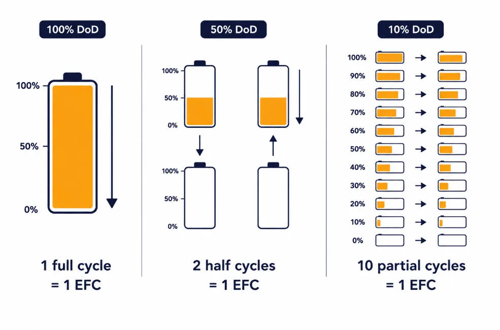
EFC has one well-known limitation: it treats every amp-hour the same, no matter how deep the swing was. As Energy-Storage.News notes, EFC alone cannot tell one cycle at 100% depth of discharge apart from two cycles at 50% DoD, or ten cycles at 10% DoD. Yet these three patterns stress the cell chemistry quite differently. So, shallow frequent cycling and deep infrequent cycling can log an identical EFC number. Even so, they age the pack at very different rates.
Many BMS platforms partly correct for this. They re-base the EFC denominator against current estimated capacity instead of nameplate capacity. That keeps the figure accurate as the pack fades. Even so, the core blind spot remains. This gap is exactly what rainflow-based BMS cycle counting was built to close.
4. Method 3: Rainflow-Based BMS Cycle Counting for Partial Cycles
Rainflow counting began as a tool for mechanical fatigue analysis. Engineers used it to turn a noisy load history into a clean set of discrete stress cycles. Battery researchers later adapted the same logic for SOC traces. A peer-reviewed ScienceDirect study on grid-integrated BESS cycle counting confirms it as the most widely used cycle-counting algorithm in the field today. Rainflow-based BMS cycle counting solves what EFC cannot: it identifies the depth of every individual swing, not just the running total.
How the Rainflow Algorithm Works Step-by-Step
The BMS records every local extremum in the SOC trace. In other words, it logs every point where the pack switches from charging to discharging, or back again.
It then calculates the SOC delta between each set of three consecutive extrema.
Consequently, If the middle delta is smaller than or equal to both neighbours, that segment counts as one closed, complete cycle at that specific depth.
The BMS removes those two points. Then it repeats the comparison on the remaining trace — much like water draining off a stepped rooftop, which is where the algorithm gets its name.
The output is a list of discrete cycles, each tagged with its own depth of discharge. For example: “47 cycles at ~80% DoD, 1,200 cycles at ~15% DoD,” instead of one flattened EFC figure.
One detail matters here: rainflow-based BMS cycle counting applies to depth of discharge, not absolute SOC. A swing from 80% down to 70% and a swing from 20% down to 10% both register as the same 10%-DoD event. Both count as equivalent stress. This lines up with how degradation models actually work, since most treat wear as a function of cycle depth, not the absolute SOC band it happens in.
Because rainflow output preserves depth data, it feeds straight into the DoD-weighted models used by SOH and RUL algorithms. That is the same layer we cover in our guide to BMS algorithms explained.
5. Method 4: Stress-Weighted BMS Cycle Counting
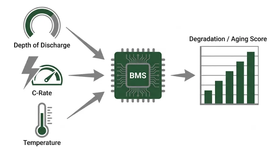
The most advanced BMS and EMS platforms push rainflow-based BMS cycle counting one step further. Instead of tallying cycles by depth alone, each identified cycle passes through a stress function. That function also factors in the C-rate and cell temperature present during that specific cycle. For instance, a 60%-DoD cycle at 0.2C and 25°C is far gentler than the same 60%-DoD cycle at 1.5C and 40°C. A stress-weighted counter reflects that difference clearly.
Rather than reporting a raw cycle count, this method builds a running “degradation” or “aging” score. That score, not the raw EFC number, feeds the most accurate RUL models. This is also why two BESS units with an identical EFC count can end up with very different projected remaining life.
6. How Firmware Filters Noise Before BMS Cycle Counting Begins
Raw current-sensor data is noisy. Grid-frequency jitter, brief EMS corrections, and normal sensor tolerance all create tiny, meaningless direction reversals in the SOC trace. Sometimes there are hundreds per hour. Feed that data straight into a rainflow algorithm, and the result is an explosion of trivial micro-cycles. Those micro-cycles overstate wear.
To prevent this, production BMS cycle counting firmware applies a minimum-delta, or hysteresis, threshold. A direction reversal only counts as a genuine local extremum once SOC has moved by some minimum amount, commonly 1–2%. Only then does it enter the counting algorithm. Firmware treats smaller reversals as noise and ignores them.
This single design choice separates a BMS that produces warranty-defensible cycle data from one that does not. Set the threshold too low, and cycle counts inflate from sensor noise. Set it too high, and the BMS misses genuine shallow cycling that still adds to ageing. Therefore, always ask your BMS supplier what hysteresis threshold their firmware applies. Datasheets rarely publish this figure. Yet it directly shapes every downstream SOH and warranty number.
7. Comparing the Four Cycle-Tracking Methods
Method
What It Captures
DoD-Aware?
Best For
Main Limitation
Threshold counting
Full 95%–5% traverses only
No
Simple consumer packs
Badly undercounts partial-cycling BESS
Ah-throughput (EFC)
Cumulative current throughput
No
Warranty reporting, simple dispatch
Cannot distinguish deep vs. shallow cycling
Rainflow counting
Each discrete swing, by depth
Yes
SOH modelling, mixed dispatch profiles
More compute-intensive; needs clean extrema
Stress-weighted counting
Depth + C-rate + temperature
Yes
RUL prediction, warranty defensibility
Requires a validated stress model per cell type
Most premium BMS platforms do not rely on just one method. Instead, they report EFC for simple dashboards and warranty tracking. Meanwhile, they run rainflow and stress-weighted BMS cycle counting in the background to feed SOH and RUL models. If a supplier says their BMS “counts cycles” without naming a method, ask directly. The gap between threshold counting and stress-weighted rainflow counting can differ by an order of magnitude in reported wear.
8. Why Datasheet Numbers Rarely Match Real-World Wear
A supplier’s “6,000 cycles to 80% SOH” claim is almost always a lab-derived EFC figure. Labs measure it under fixed, controlled conditions. That means a specific depth of discharge, often 80–90%, a specific C-rate, often 0.5C–1C, and a specific ambient temperature, often 25°C. Change any one of these variables in the field, and the real cycle-life outcome shifts. Sometimes it shifts substantially. We cover this relationship in detail in our guide to how temperature affects LFP battery cycle life. You can also model your own scenario with our battery cycle life calculator. For a broader reference on stationary lithium battery testing conditions, see IEC’s battery safety and performance standards.
In practice, your BMS’s in-field EFC or rainflow-weighted count measures a different operating profile than the datasheet number. A BESS running frequent shallow cycles at moderate temperature may outlive its rated cycle count in calendar terms. Meanwhile, one running deep cycles at high ambient temperature may fall short of it. Neither outcome means the datasheet number was wrong. It simply means BMS cycle counting and lab-rated cycle life measure two related, but distinct, things.
9. Questions to Ask About Your Supplier’s BMS Cycle Counting Method
Which cycle-counting method does the firmware run: threshold, raw EFC, rainflow, or stress-weighted? A BMS that only reports raw EFC cannot show how deep-cycling patterns affect real degradation.
What minimum-delta, or hysteresis, threshold filters noise before a reversal counts as a cycle? An unpublished or unreasonably low threshold can quietly inflate cycle counts.
Is the EFC denominator based on nameplate capacity or current estimated capacity? Using nameplate capacity for the pack’s whole life understates EFC as the cell ages.
Does the cycle-counting output feed the SOH and RUL algorithms directly, or are they calculated separately? Disconnected pipelines often cause inconsistent SOH and warranty reporting.
What DoD, C-rate, and temperature conditions does the warranty’s rated cycle-life figure assume? This baseline is what your field cycle count should be compared against, not treated as a universal number.
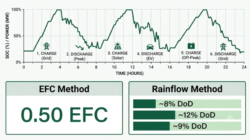
Consider a 100 kWh BESS module running a frequency-regulation profile for one day. It discharges 8 kWh, charges 5 kWh, discharges 12 kWh, charges 10 kWh, discharges 6 kWh, and charges 9 kWh. That adds up to 50 kWh of cumulative throughput.
Decomposed into 3 discrete cycles at ~8%, ~12%, ~9% DoD
3 shallow cycles logged, none flattened into one number
While both numbers are technically correct, they answer different questions. The 0.50 EFC figure shows up on a simple throughput dashboard and feeds warranty-cycle tracking. The rainflow breakdown, however, is what a SOH model actually needs. Three shallow 8–12% DoD cycles age a cell differently than one 50%-DoD cycle would. That holds true even though both scenarios can produce the same EFC total.
Conclusion: BMS Cycle Counting Is a Modelling Choice, Not a Simple Tally
A BMS does not count cycles the way a person counts laps around a track. Instead, it reconstructs a cycle metric from a continuous current and SOC trace. Each method trades simplicity for accuracy differently. Threshold counting is too crude for real BESS dispatch. EFC is the industry-standard warranty metric, yet it stays blind to depth of discharge. Rainflow-based BMS cycle counting recovers that missing depth information. It breaks messy, real-world SOC traces into discrete, weighted cycles. Stress-weighted counting goes further still. It folds in C-rate and temperature to build the aging score that actually drives accurate RUL prediction.
For BESS buyers and operators, the lesson is simple. Do not take “the BMS tracks cycle count” at face value. Instead, ask which method it uses. Ask how it filters sensor noise. And ask how that number connects to the SOH and RUL figures you will eventually rely on for warranty claims and second-life valuation.
☀️ Need a BMS Cycle Counting and SOH Methodology Review? SunLith Energy reviews BMS cycle counting implementation, EFC and rainflow methodology, and SOH-RUL linkage for BESS projects from 50 kWh upward. Contact us before you commit to a supplier.
Frequently Asked Questions
How does BMS cycle counting work?
BMS cycle counting converts raw current and SOC data into a wear metric. Most systems first calculate cumulative Ah or kWh throughput. They then convert it into Equivalent Full Cycles. More advanced platforms add a rainflow algorithm on top. It breaks the SOC trace into discrete cycles at their true depth of discharge, filtering out small reversals below a set noise threshold.
What is an Equivalent Full Cycle (EFC) in BMS cycle counting?
An EFC is the standard unit behind most BMS cycle counting for warranty purposes. The BMS sums all Ah or kWh throughput — every unit of charge or discharge, in either direction. It then divides that total by the pack’s rated or current estimated capacity. Two cycles at 50% depth of discharge, and one cycle at 100% depth of discharge, both produce 1 EFC.
Why does depth of discharge matter if EFC already tracks total throughput?
Because EFC only tracks the total charge moved, not how it was distributed. A cell that goes through one deep 100%-DoD cycle experiences different stress than one that goes through ten shallow 10%-DoD cycles. Yet both can produce the same EFC total. Rainflow-based BMS cycle counting exists specifically to preserve this depth information for accurate SOH and RUL modelling.
What is rainflow counting, and why does BMS cycle counting use it?
Rainflow counting is an algorithm first built for mechanical fatigue analysis. Applied to a battery’s SOC trace, it identifies local turning points. It then pairs them into discrete, complete cycles at their true depth of discharge, instead of one flattened throughput number. This makes it the preferred method for BMS cycle counting on BESS platforms with irregular, partial-cycling dispatch profiles.
Why doesn’t my BESS ever seem to reach the cycle count on its datasheet?
The datasheet figure is almost always measured under fixed lab conditions: a specific depth of discharge, C-rate, and temperature. If your system cycles more shallowly, at a gentler C-rate, or at cooler temperatures, its real-world BMS cycle counting output accumulates more slowly than the lab figure implies. The reverse is true under harsher conditions.
Can two BESS units show the same cycle count but have different remaining life?
Yes. Raw EFC, and even simple cycle counts, do not capture the temperature and C-rate conditions each cycle occurred under. This is why advanced BMS cycle counting adds a stress-weighted layer. It produces a degradation score rather than a plain cycle number, which feeds more accurate Remaining Useful Life predictions than cycle count alone.
BESS oversizing — deliberately installing more nameplate energy capacity than your immediate load demands — is one of the most debated decisions in battery storage project design. Therefore, getting this decision right has direct consequences for project ROI, battery longevity, and contracted performance guarantees. Furthermore, as storage markets mature and the Section 48E Investment Tax Credit continues to reshape project economics, understanding when BESS oversizing helps and when it hurts has never been more important.
In this guide, we break down the real pros and cons of BESS oversizing across residential, commercial and industrial (C&I), and utility-scale applications. Additionally, we provide a practical sizing framework, a direct comparison with the augmentation alternative, and clear guidance on how much oversizing is appropriate for each use case. For background on key BESS performance metrics, see our BESS specifications guide.
Key Takeaway BESS oversizing reduces average depth of discharge, extends cycle life, and provides a degradation buffer — but it carries real costs in capex, idle capacity, and calendar aging risk. Consequently, the right answer depends entirely on your use case, load profile, battery chemistry, and project economics.
What Is BESS Oversizing? Definition and Key Drivers
BESS oversizing means installing more nameplate energy capacity (kWh) or power capacity (kW) than the system is expected to dispatch on a daily basis under normal operating conditions. In other words, it is the deliberate act of selecting a battery system larger than the immediate load or solar coupling requirement.
The Four Main Reasons Projects Choose BESS Oversizing
Project developers and system designers choose BESS oversizing for four primary reasons. First, it provides a built-in degradation buffer — batteries lose capacity over time, so installing extra kWh upfront ensures the system still meets its contractual output at end of life (EOL). Second, it reduces the average depth of discharge (DoD), which significantly reduces electrochemical stress and extends cycle life. Third, it future-proofs the system against load growth — a facility adding EV chargers or expanding solar may outgrow a precisely sized BESS within three to five years. Finally, the ITC captures a larger credit on the full installed capacity at commissioning rather than on augmented modules added later.
BESS Oversizing vs Augmentation: Two Different Strategies
It is important to separate two strategies that are frequently conflated: oversizing (installing more capacity upfront) and augmentation (adding capacity later). Both address the degradation problem, but they carry very different economic and technical profiles. Whereas oversizing locks in capex on Day 1, augmentation defers cost — but at the risk of losing ITC eligibility on the additional modules. We explore this comparison in detail in Section 5.
Pros of BESS Oversizing: 7 Technical and Financial Benefits
1. Extended Cycle Life Through Lower Depth of Discharge
The single most significant technical benefit of BESS oversizing is the reduction in average Depth of Discharge (DoD). Battery cycle life is acutely sensitive to DoD: a LiFePO4 (LFP) cell discharged to 80% DoD typically delivers 3,000–6,000 cycles to 80% capacity retention, whereas the same cell cycled at 40% DoD can exceed 10,000 cycles. Moreover, for NMC chemistry, the spread is even wider. Therefore, oversizing directly reduces the daily DoD, keeping cells in the shallow-cycle, high-longevity operating zone. As a result, the total useful life of the system increases substantially — without any hardware change.
A peer-reviewed sizing study published in MDPI Energies confirmed that an oversized BESS consistently operates at approximately 30% DoD, significantly reducing cycling degradation compared to a precisely sized system. See our BESS cycle life comparison guide for detailed 0.5C vs 1C cycling data across liquid-cooled LFP formats.
2. Built-In Degradation Buffer for End-of-Life Performance
All BESS contracts and revenue agreements are written against end-of-life capacity, not nameplate. Consequently, a project designed to deliver 1 MWh at year 10 must either oversize at commissioning to absorb predicted capacity loss, or augment mid-life. BESS oversizing solves this directly: the 15–20% extra capacity at year 0 becomes the system’s normal operating capacity at year 8–10, after degradation has run its course. In addition, oversizing also enables developers to lock in capital expenditures at project outset, mitigating future cost uncertainty. For a deeper understanding of capacity fade mechanics, see our Battery State of Health (SoH) estimation guide.
3. Improved Round-Trip Efficiency at Partial Loads
Battery inverters and Power Conversion Systems (PCS) operate most efficiently when working well below their rated power ceiling. Therefore, an oversized BESS means the power electronics run at partial load more often, reducing switching losses and thermal stress. Across LFP systems, round-trip efficiency (RTE) typically reaches 90–95% in well-managed partial-load conditions versus 85–88% when the system is pushed to rated limits daily. Furthermore, professional system sizing guidelines recommend oversizing by 5–20% specifically to compensate for RTE losses over the project’s lifetime. For a full breakdown of how RTE impacts your PCS selection, visit our BESS PCS functions and features guide.
4. Future-Proofing for Load Growth
Commercial and industrial facilities are rarely static. An EV fleet charging infrastructure build-out, a new production line, additional HVAC loads, or expanded solar capacity can all push a precisely sized BESS into insufficiency within a few years. As a result, BESS oversizing provides headroom to absorb load growth without a full system redesign or costly inverter upgrades. For residential customers, similarly, oversizing by 10–20% accounts for future appliance electrification — heat pumps, EV charging, induction cooking — that increase household energy consumption over time. This is especially relevant given that electricity rates have increased 32% over the past decade and the trend is expected to continue.
5. Greater Resilience During Extended Outages
An oversized BESS provides substantially longer backup durations during grid outages. For instance, where a precisely sized system may sustain critical loads for 4–6 hours, a 25% oversized system of the same power rating extends that window to 5–7.5 hours without additional hardware. Consequently, for hospitals, data centres, manufacturing facilities, and off-grid microgrids, this resilience buffer is a core design requirement rather than an optional feature. In addition, BESS oversizing enables higher solar self-consumption ratios, because the system can absorb more excess PV generation that would otherwise be curtailed — especially in DC-coupled configurations. Our cylindrical vs prismatic LFP cell guide covers how cell format selection interacts with resilience design.
6. Tax Credit Maximisation Under Section 48E
Under the Section 48E Clean Electricity Investment Tax Credit, the ITC applies to the full installed nameplate capacity at commissioning. Projects beginning construction before 2033 can qualify for a base credit of 6% rising to 30% — or up to 50% with domestic content and labour standards — on the entire installed system. Therefore, oversizing at commissioning rather than augmenting later allows developers to capture ITC on the additional capacity now, when the credit is at its most generous. As documented by Energy-Storage.News, Pivot Energy uses optimisation models specifically to find the ‘sweet spot’ where overbuilding by 15–20% captures the full ITC while also reducing DoD and slowing the degradation curve.
7. Higher Solar Self-Consumption and Clipping Capture
In solar-plus-storage configurations, an oversized BESS absorbs more excess PV generation that would otherwise be curtailed — particularly in DC-coupled systems where the battery captures inverter clipping losses. Projects with aggressively sized solar arrays consequently benefit most from an oversized storage buffer, enabling higher self-consumption ratios and better time-of-use (ToU) arbitrage revenue. Additionally, the flat voltage profile of LFP cells means the battery can accept charge across a wider SoC range without significant efficiency loss, making it well-suited to absorbing variable clipping events.
Cons of BESS Oversizing: 7 Real Drawbacks to Weigh
1. Higher Upfront Capital Expenditure
The most obvious downside of BESS oversizing is cost. At current commercial LFP BESS pricing of $220–$320 per kWh (nameplate, installed), adding 15–25% extra capacity translates directly into a 15–25% larger capital outlay. For example, on a 1 MWh C&I project, the oversizing premium reaches $33,000–$80,000. On a 10 MWh utility-scale project, the figure climbs to $330,000–$800,000. As a result, higher capex extends payback periods, dilutes IRR, and increases financing costs. Moreover, the 20/80 rule for battery SoC management — explored in our 20/80 rule for batteries guide — shows that moving from a 90% DoD strategy to a strict 60% DoD strategy for the same usable energy requires installing roughly 33% more nameplate capacity, at a steep capex premium.
2. Idle Capacity — Stranded Capital
An oversized BESS, by definition, contains capacity that is not used every day. In a system with a 30% oversizing factor, approximately 23% of the installed kWh is functionally stranded under normal operating conditions — generating no direct revenue, not contributing to peak shaving, and not offsetting grid draw. Therefore, for merchant revenue projects where every kWh of contracted discharge must justify its hardware cost, idle capacity directly weakens the financial case. Consequently, a detailed financial model comparing oversized vs precisely sized scenarios is essential before committing to an aggressive oversizing strategy.
3. Calendar Aging at High State of Charge
There is a subtle but real risk in BESS oversizing: a battery that is rarely deeply discharged will consequently spend more time at a high state of charge (SoC) between cycles. For LFP, this matters less due to the flat voltage curve, but for NMC and NCA chemistries, sustained high SoC accelerates calendar aging through lithium plating and electrolyte decomposition. The EMS must therefore be configured with SoC upper limits (typically a 90% ceiling) to mitigate this risk, which further reduces the usable window — partially negating the oversizing benefit.
4. Larger Physical Footprint and Permitting Complexity
A larger BESS means more rack space, additional container units, larger electrical rooms, and more complex fire suppression under NFPA 855 setback requirements. For urban C&I projects, rooftop installations, or sites with constrained footprints, BESS oversizing may simply not be feasible without additional civil and structural engineering. As a result, the incremental cost of accommodating a larger system can erode or eliminate the economic benefit of the additional capacity.
5. Risk of Over-Engineering Against Inaccurate Load Projections
BESS oversizing is typically justified by load growth projections that may not materialise. A facility forecasting 30% energy consumption growth over five years but actually growing 10% has paid a significant capex premium for capacity that will never be fully utilised. Furthermore, the further into the future the projections extend, the less reliable they become — and the weaker the economic case for aggressive oversizing. Therefore, right-sizing discipline, grounded in real interval load data, is essential before committing to an oversizing strategy.
6. Interconnection Limit Conflicts
Utility interconnection agreements define the maximum allowable power at the Point of Common Coupling (PCC). An oversized BESS that exceeds the permitted inverter or PCS rating — or that pushes a project over the interconnection ceiling — may require expensive distribution upgrades, transformer replacements, or grid impact studies. As a result, always validate that the oversized system’s power rating remains within interconnection constraints before finalising the design.
7. Diminishing Returns on ROI for Thin-Margin Projects
For projects where the economics are already marginal — low ToU spreads, limited demand charges, or thin merchant power prices — the additional capex of BESS oversizing may not be recoverable within the project’s financial life. Therefore, a right-sizing discipline, rather than aggressive oversizing, often produces better risk-adjusted returns on projects operating in challenging market conditions. Additionally, if battery prices continue to fall, augmentation at year 5–7 may deliver the same EOL capacity guarantee at a lower total lifecycle cost than oversizing today.
BESS Oversizing Pros and Cons: Quick-Reference Comparison Table
PROS of BESS Oversizing
CONS of BESS Oversizing
Extends cycle life by reducing average DoD
Higher upfront capital expenditure
Slower capacity degradation over project lifetime
Idle capacity — underutilised asset
Buffer for future load growth without re-powering
Larger footprint and space requirements
Improves round-trip efficiency at partial loads
Additional BMS / thermal management complexity
Strengthens resilience during extended outages
Risk of battery sitting at high SoC, accelerating calendar aging
Lock in ITC / 48E tax credits on full capacity now
Diminishing returns if load growth projections are wrong
Reduces depth of discharge and thermal stress
Potentially overshoots interconnection limits
Supports higher solar self-consumption
Makes ROI harder to justify on thin-margin projects
BESS Oversizing vs Augmentation: Which Degradation Strategy Wins?
The BESS oversizing debate is inseparable from its primary alternative: augmentation — the strategy of adding battery modules at year 5 or 7 to restore degraded capacity. However, these strategies are not equivalent, and the right choice depends on several project-specific factors.
Factor
BESS Oversizing (Upfront)
Augmentation (Mid-Life)
Capex Timing
Higher Day-1 cost; lower total lifecycle cost
Lower Day-1 cost; uncertain future capex at year 5–7
ITC Eligibility
Full credit on entire capacity at commissioning
Augmented capacity may miss ITC or face FEOC risk
Degradation Benefit
Reduces DoD and slows degradation from Day 1
Addresses degradation after it has occurred
Space Planning
Must install full footprint upfront
Must reserve physical and electrical space for future modules
Falling Battery Prices
Locks in today’s cost for future capacity
May benefit from lower prices at year 5
Complexity
Lower operational complexity
Requires mid-project procurement and system rebalancing
C&I with budget constraints; markets with falling storage prices
As battery prices continue to fall, augmentation is becoming more attractive for some project types. Nevertheless, as Pivot Energy’s modelling demonstrates, for ITC-sensitive projects, oversizing by 15–20% upfront typically produces better risk-adjusted NPV than augmentation — particularly given the difficulty of qualifying augmented capacity for the same ITC rate under the One Big Beautiful Bill Act.
How Much BESS Oversizing Is Right? A Use-Case Sizing Guide
There is no universal BESS oversizing percentage. Instead, the right buffer depends on your use case, battery chemistry, load profile, and project economics. However, the table below provides a practical reference framework covering the most common project types:
Use Case
Recommended BESS Oversizing
Rationale
Key Risk if Under-Sized
Residential Solar + Storage
10–20%
Compensate for DoD and RTE losses; buffer seasonal variation
Example: 30 kWh/day load × 2 autonomy days = 60 kWh base ÷ 0.85 DoD × 0.92 RTE = 76.6 kWh nameplate minimum + 15% degradation buffer = approximately 88 kWh recommended nameplate capacity
Note: For LFP chemistry with a 90% DoD operating window, adjust DoD factor accordingly.
For LFP chemistry specifically, the degradation benefit of BESS oversizing is more modest than for NMC or NCA, because LFP already exhibits a flatter voltage curve and superior cycle life at high DoD. Therefore, the most rigorous approach — as recommended in NREL’s Energy Storage Modelling guidelines and the IEA’s Batteries and Secure Energy Transitions report — is to use simulation tools such as NREL’s SAM or PVsyst with real 15-minute interval load data to determine the optimal capacity that minimises LCOE while meeting the contracted capacity guarantee at EOL.
Does Battery Chemistry Change the BESS Oversizing Calculus?
Yes — significantly. However, the extent to which BESS oversizing is beneficial varies considerably by chemistry. Here is how the most common BESS chemistries interact with oversizing strategy:
LFP (LiFePO4): The Most Common Choice for Commercial BESS
LFP already offers exceptional cycle life — 6,000–10,000+ cycles at 0.5C to 80% SoH — a flat voltage curve that reduces SoC-related aging, and thermal stability above 270°C. Therefore, the benefit of BESS oversizing for LFP is real but more modest than for NMC. A 10–15% oversizing factor is typically sufficient for residential and C&I LFP projects, unless extended autonomy is a primary requirement. For a detailed comparison of LFP cell formats, see our cylindrical vs prismatic LFP guide.
NMC (Nickel Manganese Cobalt): Greater Benefit from Oversizing
NMC cells are more sensitive to both high SoC and high DoD. The cycle life penalty for deep discharging is steeper, and calendar aging at high SoC is more pronounced. Consequently, for NMC-based systems, BESS oversizing by 20–30% can provide meaningful cycle life extension. However, the EMS must be configured to avoid sustained high-SoC parking, which otherwise accelerates precisely the degradation the oversizing was intended to prevent.
NCA (Nickel Cobalt Aluminium): Strongest Case for Oversizing
NCA is even more sensitive to DoD extremes than NMC. Therefore, BESS oversizing is strongly recommended for NCA systems, alongside strict SoC window management — typically a 20–90% operational band. As a result, NCA-based utility-scale systems frequently carry 20–30% oversizing factors as a standard design requirement.
When to Choose BESS Oversizing — and When to Avoid It
Oversize Your BESS When These Conditions Apply
Your project carries a 10+ year contract or PPA with capacity guarantee provisions that must be met at end of life
You are qualifying for ITC / Section 48E and want to maximise the tax credit on the full installed capacity at commissioning
The site has a clear load growth trajectory — EV charging, electrification roadmap, or solar expansion planned
You are designing an off-grid or critical backup system where autonomy days are non-negotiable
NMC or NCA chemistry is specified and DoD reduction delivers a significant cycle life benefit
Your DC-coupled solar array is oversized relative to the inverter and the battery can capture clipping energy
The incremental capex of BESS oversizing is recoverable within the project financial model
Avoid BESS Oversizing When These Conditions Apply
Project economics are already thin and additional capex pushes IRR below the acceptable threshold
Load forecasts are highly uncertain and growth projections lack solid 15-minute interval data support
Physical space constraints make a larger system impractical or disproportionately expensive to install
The interconnection agreement caps power capacity at a level that already constrains daily dispatch
Battery prices are falling rapidly in your market and augmentation in year 5–6 will be substantially cheaper
LFP chemistry is specified and daily DoD is already inherently low (below 60%) with proper sizing
The Four-Step BESS Oversizing Decision Framework
Rather than guessing at an oversizing percentage, use this structured four-step framework to determine whether BESS oversizing is appropriate for your project and, if so, by how much. As a result, you will arrive at a defensible, financially grounded nameplate capacity rather than an arbitrary rule of thumb.
Step 1 — Load Analysis: Gather Real Interval Data
First, collect at least 12–24 months of 15-minute interval load data. Identify peak demand events, average daily consumption, and seasonal variation patterns. This step is non-negotiable: BESS oversizing justified by rough annual consumption estimates rather than interval data almost always produces either over-engineered or under-performing systems.
Step 2 — Base Capacity Calculation
Next, apply the standard sizing formula — daily load × autonomy days ÷ (DoD × RTE) — to establish the minimum required nameplate capacity. This gives you the floor, not the target. However, it also reveals exactly how sensitive the result is to your DoD and RTE assumptions.
Step 3 — Apply Chemistry and Use-Case Correction
Subsequently, determine your oversizing factor based on battery chemistry (LFP vs NMC vs NCA), use case (peak shaving vs backup vs grid services), and EOL capacity requirement. Reference the sizing guide table in Section 6 for starting-point percentages, then adjust based on site-specific factors including climate, cycling frequency, and interconnection limits.
Step 4 — Financial Validation: Model Both Scenarios
Finally, model the oversized vs precisely sized scenarios in a full project NPV and IRR analysis, incorporating ITC capture, degradation trajectory, load growth assumptions, and augmentation cost projections. As a result, you will arrive at the scenario that maximises risk-adjusted return while meeting contracted performance obligations. Choose the strategy with the superior risk-adjusted NPV — not the one that simply installs the most battery.
Conclusion: BESS Oversizing Is a Strategy, Not a Default
BESS oversizing is one of the most powerful tools in a storage developer’s arsenal — but only when applied with precision. When the economics support it, oversizing by 10–25% delivers longer cycle life, a built-in degradation buffer, greater resilience, higher solar self-consumption, and maximised ITC capture. Conversely, when applied without a sound load analysis and financial model, it simply commits capital to cells that will never discharge.
The right approach is always project-specific. Therefore, an LFP C&I peak shaving project with a 10-year capacity guarantee may need 15–20% BESS oversizing to meet EOL targets. A residential grid-tied backup system with low daily DoD requirements may need only 10%. An off-grid microgrid with strict autonomy requirements and no grid fallback may need 25–30%. Furthermore, as battery prices continue to fall, the break-even point between oversizing and augmentation will shift — making it essential to rerun the financial model on each new project rather than applying a fixed rule.
At Sunlith Energy, every BESS project we design goes through a rigorous sizing and degradation modelling process — using real interval load data, validated chemistry models, and financial sensitivity analysis. To learn more about how we approach BESS design, explore our BESS specifications guide, our Battery SoH estimation guide, or review the NREL Grid-Scale Battery Storage Technology Basics for independent technical context. The goal is never the largest battery — it is the right battery, sized correctly for your project’s lifetime.
Ready to size your BESS correctly? Contact the Sunlith Energy team for a technical consultation. We combine 14+ years of LiFePO4 expertise with advanced degradation modelling to design storage systems that perform at end of life, not just on commissioning day.
The 20/80 rule for batteries is one of the most repeated tips in battery care. It is also one of the most misunderstood. Open any EV forum or BESS manual, and you will read the same line. Keep the battery between 20% and 80% state of charge.
For lithium-ion batteries, the 20/80 rule sets a charging window. It avoids the two extremes of state of charge (SoC) that speed up wear. Stay above 20% SoC. Stay below 80% SoC. Do that, and the battery lasts longer. This applies to a phone, an EV, or a multi-megawatt BESS alike.
But for BESS buyers, the 20/80 rule raises a hard question. If 60% of capacity is the “safe zone,” what happens to the rest? Is 40% just stranded capital, sitting idle in a container? And does a rule built for phones and EVs even fit a grid-connected LFP system, built for daily cycling over 15 to 20 years?
This guide answers that question from first principles. First, we cover the electrochemistry behind the rule. Next, we compare it with other SoC windows. Then, we look at how chemistry and BMS design change the picture. Most importantly, we ask whether the cycle life gains are worth the lost capacity in real BESS projects.
1. What Is the 20/80 Rule for Batteries?
The Basic Definition
State of charge (SoC) measures how much energy a battery holds right now. It is shown as a percentage of usable capacity. A battery at 100% SoC is full. A battery at 0% SoC has hit its lower cutoff. That cutoff is not zero volts, though. The BMS always keeps a safety margin below it.
In short, the 20/80 rule means one thing. Keep charging and discharging inside the 20% to 80% SoC band. Do not let the battery swing from empty to full on every cycle. As a result, the operating window equals 60% of usable capacity.
Here is the formula, stated plainly:
Formula — the 20/80 rule for batteries: Effective Depth of Discharge (DoD) = Upper SoC limit − Lower SoC limit 20/80 rule → Effective DoD = 80% − 20% = 60% A battery cycled strictly within 20–80% SoC never exceeds a 60% depth of discharge on any single cycle, regardless of nameplate capacity.
The 20/80 Rule Is Not a Safety Limit
It helps to separate the 20/80 rule from the absolute safety limits set by the Battery Management System (BMS). The BMS hard cutoffs sit close to 0% and 100%, on the cell’s true voltage range. These exist for one reason: to stop over-charge and over-discharge events that cause safety failures.
Those safety limits are not arbitrary, either. They trace back to formal standards such as IEC 62619, which sets safety requirements for industrial lithium battery systems. The 20/80 rule, by contrast, operates well inside those hard limits. It is simply a usage strategy for longevity, not a safety boundary.
The table below shows how SoC windows map to depth of discharge. This is the same language used on every BESS datasheet.
2. The Science Behind the 20/80 Rule for Batteries
Why does the 20/80 rule exist at all? The answer sits inside the cell. Specifically, it comes down to what happens physically at the extremes of state of charge.
Why High SoC (Above 80%) Speeds Up Degradation
As a cell nears full charge, the cathode reaches peak lithium depletion. Voltage peaks too. As a result, this high-voltage state strains the cathode’s crystal lattice. Over many cycles, that strain adds up to real structural wear.
At the same time, the electrolyte faces its highest oxidative stress near full charge. This, in turn, speeds up electrolyte breakdown. It also drives further growth of the solid electrolyte interphase (SEI) layer on the anode.
The SEI layer is a thin film that forms naturally on the anode. In small amounts, it is actually useful. It protects the anode from further reaction with the electrolyte. However, SEI growth consumes active lithium over time. It also raises internal resistance. Because SEI growth depends heavily on voltage and temperature, both factors climb when a cell sits near 100% SoC, especially during storage.
Why Low SoC (Below 20%) Also Speeds Up Degradation
At the other extreme, very low SoC pushes the cell close to its minimum voltage cutoff. This raises the risk of copper dissolution from the anode’s current collector. The risk grows further still if the cell drifts below its minimum voltage during storage, through normal self-discharge.
Repeated deep discharges add a different kind of stress, too. On the next charge, lithium ions must fully repopulate the lattice. This places real mechanical strain on the cathode.
This is not just theory. A widely cited 2023 study on Tesla lithium-ion cells tested several SoC windows. The pattern was clear. Cells held at very high or very low SoC degraded faster than cells held at moderate SoC. Notably, the shortest service life showed up in cells cycled below 25% SoC.
The Electrochemical “Sweet Spot” in the Middle
Between these two extremes sits a calmer stretch of the voltage curve. Here, both electrodes face comparatively low stress. This, in fact, is the electrochemical basis for the 20/80 rule. By skipping the top and bottom 20% of the SoC range, a battery spends its life in the zone where SEI growth, electrode strain, and electrolyte oxidation all move slowest.
Separately, research into partial state of charge (PSoC) cycling backs this up further. Cycle life improves when a fixed amount of charge is cycled from a partial state, rather than from full charge. One widely referenced study confirmed this directly. The effect grew stronger still when depth of discharge was also reduced. In effect, this is the scientific backbone of the 20/80 rule, applied right at the cell level.
3. The 20/80 Rule for Batteries vs Other SoC Windows
The 20/80 rule is the most common SoC window in consumer guidance. But it is not the only one in use. BESS specs, EV guidance, and standby power systems each favour slightly different windows. The right choice depends on how usable capacity and cycle life get weighted for that specific application.
How the 20/80 Rule for Batteries Compares to Other SoC Windows
SoC Window
Effective DoD
Relative Cycle Life Impact
Usable Capacity Retained
Typical Use Case
0–100%
100%
Baseline (shortest cycle life)
100%
Maximum-capacity applications; rarely recommended for daily cycling
10–90%
80%
Moderate improvement over 0–100%
80%
Grid-scale LFP BESS, EV daily-use presets
20–80%
60%
Significant improvement; the 20/80 rule for batteries
60%
Consumer EV/phone guidance, residential storage
30–70%
40%
Maximum improvement for calendar aging
40%
Long-term standby SoC, seasonal storage, shipping
Two Patterns Worth Noting
First, SoC window width and cycle life do not scale in a straight line. The jump from 0–100% to 10–90% brings a meaningful gain. But the next jump, from 10–90% to 20–80%, brings a smaller gain. This holds true even though both moves cut DoD by 20 points.
Second, the 30/70 window rarely gets used for daily cycling. It simply gives up too much usable capacity. Instead, it works best as a storage SoC — the level a battery should sit at when idle for weeks or months. During storage, calendar aging drives degradation, not cycling.
Why BESS Often Defaults to 10–90% Instead
For BESS specifically, the 10–90% window has become the common middle ground for LFP systems. Here is why. LFP’s flat voltage curve, covered in Section 5, makes the gain from 10–90% to 20–80% quite small. Meanwhile, that extra 10% of usable capacity carries real commercial value.
4. How the 20/80 Rule for Batteries Affects BESS Sizing
Every BESS datasheet draws a line between two figures. Nameplate capacity is the total rated energy storage of the system. Usable energy is nameplate capacity multiplied by the operating depth of discharge. The SoC window sets this usable energy figure directly. As a result, it becomes one of the most consequential decisions in BESS sizing.
For more on how DoD interacts with other specs, see our guide to BESS specifications.
A Worked Sizing Example
Consider a 1 MWh nameplate BESS under three SoC strategies:
SoC Window
Effective DoD
Usable Energy (1 MWh nameplate)
“Lost” Capacity
0–100%
100%
1,000 kWh
0 kWh
10–90%
80%
800 kWh
200 kWh
20–80% (20/80 rule)
60%
600 kWh
400 kWh
On paper, the 20/80 rule strands 400 kWh out of every cycle. That is 40% of the installed asset. In practice, however, BESS designers handle this two ways.
The first approach is to oversize the nameplate capacity. This way, usable energy under the chosen SoC window still meets the project’s requirement. For example, a project needing 600 kWh of usable energy, under a 20/80 window, must size the nameplate capacity near 1 MWh, not 600 kWh.
The second approach is to accept the narrower usable energy figure instead. From day one, the dispatch strategy, tariff arbitrage, or backup duration gets designed around that smaller number. Both approaches work. The right choice depends on whether capital cost or long-term degradation is the binding constraint for that project.
Sizing Formula and Worked Example
Sizing rule of thumb: Required nameplate capacity = Required usable energy ÷ Effective DoD Example: a site needs 600 kWh of usable energy and will operate at 20/80 (60% DoD). Required nameplate capacity = 600 kWh ÷ 0.60 = 1,000 kWh (1 MWh) By comparison, the same 600 kWh requirement under a 10/90 window (80% DoD) needs only 750 kWh nameplate — a smaller, lower-cost system.
Why Warranty Terms Matter Just as Much
Warranty terms matter just as much as the SoC window itself. A BESS warranted for a set cycle count at 90% DoD reaches end-of-life on a different timeline than the same cell warranted at 60% DoD. So, always confirm which DoD figure the warranty’s cycle-life guarantee assumes. Manufacturers calculate end-of-life projections against one specific operating window, not whatever SoC range the system ends up running in practice.
5. The 20/80 Rule for Batteries by Chemistry: LFP vs NMC vs NCA vs LTO
Why NMC and NCA Are More Sensitive to SoC Extremes
The 20/80 rule did not start in the BESS industry. Instead, it became popular through consumer electronics and EV guidance, where NMC and NCA cathode chemistries dominate. These chemistries carry a steep voltage curve across the SoC range. So, small changes in SoC produce larger changes in cell voltage. That, in turn, means larger swings in the electrochemical stress covered in Section 2.
Why LFP Tolerates a Much Wider Window
LFP (Lithium Iron Phosphate) behaves quite differently. It is now the leading chemistry for stationary BESS. LFP has a notably flat voltage curve across most of its range. As a result, the voltage gap between 30% SoC and 70% SoC stays small. Compare that to an NMC cell, where the same gap is much larger. Consequently, LFP cells care less about exactly where the SoC window sits. They also tolerate the top and bottom of the range far better than NMC or NCA.
Chemistry Comparison Table
Chemistry
Voltage Curve Shape
Sensitivity to SoC Extremes
Typical Recommended Window
Common BESS DoD Spec
LFP
Flat across most of range
Low — tolerant of wide windows
5–95% (or wider)
90–95% DoD
NMC
Steep, especially at high SoC
High — benefits significantly from 20/80
20–80%
50–80% DoD
NCA
Steep, similar to NMC
High — most sensitive to high SoC
20–80%
50–80% DoD
LTO
Very flat, stable anode
Very low — minimal benefit from narrowing
0–100% viable
95–100% DoD
Why This Matters for Buyers
This is exactly why DoD specifications on commercial LFP BESS datasheets sit at 90–95%. Meanwhile, consumer guidance for NMC-based phones and EVs sticks with the much narrower 20/80 window. After all, forcing a strict 20/80 rule onto a grid-scale LFP system would strand a large slice of installed capacity. Given LFP’s flat curve, the degradation benefit simply would not justify it.
Chemistry is not the only factor that shapes how hard a cell can be pushed, though. Charge and discharge rate matters too, which we cover in our guide to BESS C-rate.
That said, the underlying principle still applies to LFP. Avoid long dwell time at very high or very low SoC, especially during idle storage. The difference is one of degree, not of kind. LFP systems can run much closer to the 0% and 100% extremes during active cycling, without the same penalty NMC or NCA cells would face.
6. How the BMS and EMS Enforce the 20/80 Rule for Batteries
In a real BESS, the 20/80 rule — or whichever SoC window applies — is not left to chance. Instead, it gets enforced through two systems working together. The Battery Management System (BMS) handles cell and pack-level protection. The Energy Management System (EMS) handles dispatch planning.
BMS-Level Enforcement: Translating SoC Limits Into Voltage Cutoffs
The BMS does not directly “see” SoC as a clean percentage. Instead, it measures cell voltage and current. From there, it estimates SoC using coulomb counting, which tracks current flow over time. This estimate then gets cross-checked against the cell’s open-circuit voltage (OCV) curve. To enforce a 20/80 window, the BMS applies soft limits. These limits map to the voltage levels tied to 20% and 80% SoC, for that specific chemistry. So, when the pack nears either limit, the BMS signals the EMS to stop charging or discharging in that direction.
Why SoC Estimation Drifts — and Why Occasional Full Cycles Matter
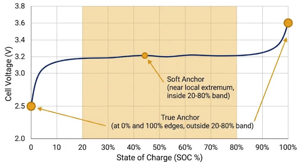
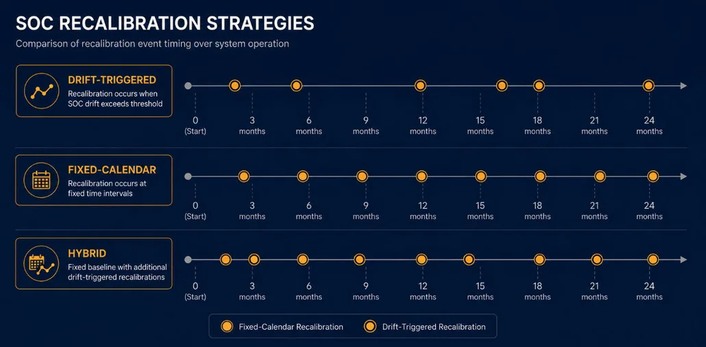
Coulomb counting builds up small errors over time. As a result, the BMS’s SoC estimate slowly drifts from the cell’s true SoC. The fix is simple, though. Periodically, the cell gets allowed to reach a known reference point on its voltage curve, typically near full charge. There, SoC can be recalibrated with high confidence.
This creates a practical tension with the 20/80 rule. A system run permanently within 20–80% SoC may see growing estimation error over months. Without occasional full-range calibration cycles, that drift only gets worse.
Fortunately, most commercial BMS platforms handle this automatically. They schedule a periodic calibration charge to a higher SoC, during a low-demand period. Then, they return to the configured operating window. This is simply a normal part of long-term SoC accuracy. It is not a violation of the SoC window strategy.
EMS-Level Enforcement: Dispatch Planning Within the Window
The BMS protects the cells from exceeding configured SoC limits. The EMS, meanwhile, plans dispatch so the battery rarely needs to hit those limits at all. A well-tuned EMS schedules charge and discharge events carefully. So, the battery’s SoC trajectory stays comfortably inside the operating window throughout a typical day. In this way, the BMS’s hard limits remain a safety backstop, not a routine operating boundary.
7. The 20/80 Rule for Batteries Across Different BESS Applications
The 20/80 rule often gets presented as a universal recommendation. In reality, though, the best SoC strategy varies a lot by application. The table below summarises how SoC strategy typically shifts, depending on use case.
Application
Typical SoC Strategy
Rationale
Residential solar + storage (NMC)
20–80% to 10–90%
Balances cycle life with daily self-consumption value; NMC benefits most from narrower windows
C&I peak shaving (LFP)
5–95% (90% DoD)
LFP’s flat voltage curve and high cycle life tolerate wide windows; ROI favours maximum usable energy
Grid-scale arbitrage (LFP)
5–95% to 0–100%
Revenue per cycle often outweighs marginal degradation cost at LFP’s cycle-life scale
Frequency regulation
Centred near 50% SoC
Symmetrical headroom needed to inject or absorb power in either direction at short notice
Backup / UPS standby
Held near 50–60% SoC
Minimises calendar aging during long idle periods between discharge events
Second-life EV battery packs (NMC)
20–80%
Already-degraded cells benefit most from the gentlest possible operating window
Frequency Regulation: Why the Middle of the Range Matters Most
Frequency regulation systems sit deliberately near the middle of their SoC range, often close to 50%. This is not really about the 20/80 rule. Instead, it is about headroom. The system must absorb or inject power within milliseconds of a frequency deviation, in either direction. A battery at 95% SoC has little room left to absorb more charge. One at 5% SoC has little room left to discharge. So, the middle of the range maximises bidirectional response capability.
Backup and UPS: A Different Kind of SoC Challenge
Backup and UPS systems face the opposite challenge. Long idle periods at a fixed SoC get punctuated only occasionally by discharge events. For these systems, the relevant guidance is less about the 20/80 rule. It is more about storage SoC — holding the battery at a moderate level, commonly 50–60%, during idle periods. This approach limits the calendar aging effects covered in Section 2. Both very high and very low storage SoC accelerate SEI growth, even when the battery just sits unused.
Off-grid and islanded systems face a related challenge, since they cannot fall back on the wider grid during a SoC excursion. For more on how that changes BESS design, see our Island Grid BESS engineering guide.
8. Quantifying the 20/80 Rule for Batteries: Cycle Life vs Capacity
Here is the central question for any BESS operator. Does the cycle life gain from a narrower SoC window actually offset the lost usable energy per cycle? The best way to compare strategies is not cycle count alone. Instead, look at total lifetime energy throughput — the cumulative kWh the system delivers before reaching end-of-life capacity.
Illustrative Throughput Comparison
The table below illustrates this trade-off for an NMC-type cell. The figures are illustrative, but they stay broadly consistent with partial state-of-charge cycling research.
SoC Window
Effective DoD
Illustrative Cycle Life (to 80% SoH)
Usable Energy per Cycle (1 MWh nameplate)
Approx. Lifetime Throughput
0–100%
100%
~2,500 cycles
1,000 kWh
~2,500 MWh
10–90%
80%
~4,000 cycles
800 kWh
~3,200 MWh
20–80% (20/80 rule)
60%
~6,000 cycles
600 kWh
~3,600 MWh
30–70%
40%
~9,000 cycles
400 kWh
~3,600 MWh
Two Things Stand Out
First, narrowing from 0–100% to 20–80% boosts lifetime throughput in a real way. In this example, the gain is roughly 44%. Second, that gain flattens out past a certain point. Moving from 20–80% to 30–70% adds many more cycles. Yet total throughput barely moves, because each extra cycle delivers proportionally less energy.
What This Means in Practice
The key insight on lifetime throughput: Total energy delivered ≈ Cycle life × Usable energy per cycle Narrowing the SoC window increases the first term and decreases the second. There is a point — often somewhere between 20/80 and 30/70 for NMC chemistries — beyond which the two effects roughly cancel out. Past that point, further narrowing mainly stretches the calendar timeline, not the total energy delivered.
This carries a direct, practical lesson. The 20/80 rule does not always mean more total energy over the system’s life. What it reliably does, instead, is spread that throughput over a longer calendar period, with lower peak stress per cycle. That matters most when calendar life, warranty terms, or thermal limits are the binding constraint, not total cycle count.
9. Is the 20/80 Rule for Batteries Worth It for BESS Buyers?
From a pure capital-cost view, every point of SoC window removed from the operating range costs something. Either more hardware gets installed to keep the same usable energy, or output gets sacrificed. At typical commercial LFP BESS costs of $220 to $320 per kWh, the math gets concrete fast.
Moving from a 90% DoD strategy to a strict 60% DoD (20/80) strategy, for the same usable energy, means installing roughly 33% more nameplate capacity. That is a substantial capex increase. And it is a steep price for a chemistry whose flat voltage curve already makes the degradation benefit fairly small.
Why LFP Buyers Should Look Beyond 20/80
The calculus changes for NMC and NCA-based systems, where the 20/80 rule’s degradation benefit runs largest. For these chemistries, the extra upfront cost of oversizing is more often worth it. The payoff is a real extension of warranty-covered service life. This matters most where replacement logistics are difficult, such as second-life EV packs or remote and offshore installations.
Tracking that degradation over time matters just as much as the SoC strategy itself. For more on how suppliers estimate remaining battery health, see our guide to DCIR-based State of Health estimation for BESS.
Three Reasons LFP Favours a Wider Window
For most grid-connected commercial and utility-scale LFP BESS, the economically optimal SoC window sits much closer to 5–95% or 10–90% than to 20/80. There are three clear reasons why:
LFP’s flat voltage curve means the marginal degradation cost of the additional 10–30% of usable energy is small.
Revenue-generating applications (arbitrage, demand charge reduction, frequency services) are typically valued per kWh cycled, so reduced usable energy directly reduces revenue.
LFP cycle life figures (3,000–8,000+ cycles to 80% SoH) already provide 10–15+ years of service even at high DoD for most daily-cycling applications.
Overall, the 20/80 rule still earns its place as a default heuristic for NMC/NCA-based systems. It also works well as a long-term storage SoC guideline, across all chemistries. And it remains a sensible starting point for buyers who do not yet have chemistry-specific degradation curves. But it should not be treated as a fixed engineering spec for LFP-dominated stationary storage. Instead, the right SoC window is chemistry-specific and application-specific, not a universal constant.
SoC strategy is just one input into overall project returns. Round-trip losses matter too, and we cover those in our guide to BESS round-trip efficiency (RTE).
10. Best Practices and Common Mistakes With the 20/80 Rule for Batteries
Best Practices
Request chemistry-specific degradation curves (cycle life vs DoD) from your cell supplier rather than relying on generic 20/80 guidance.
For LFP systems, evaluate the 5–95% or 10–90% range as the realistic operating window, reserving 20/80-style restrictions for long-term storage SoC rather than daily cycling.
For NMC/NCA-based systems — including residential storage and second-life EV packs — the 20/80 rule remains a reasonable and well-supported default.
Confirm which DoD value the manufacturer’s cycle-life warranty is based on, and ensure your operating SoC window matches that assumption.
If a system will be idle for extended periods (shipping, seasonal storage, commissioning delays), set the storage SoC to a moderate level — commonly 30–60% — regardless of the chemistry.
Allow the BMS to perform periodic full-range calibration cycles even if the operating SoC window is narrower; this maintains SoC estimation accuracy over the system’s life.
Common Mistakes
Applying consumer EV/phone-based 20/80 guidance directly to a grid-scale LFP BESS without accounting for the chemistry’s much flatter voltage curve.
Sizing a system’s nameplate capacity around a 0–100% assumption, then discovering that the operating SoC policy reduces usable energy below the project’s requirement.
Treating the 20/80 rule as a hard safety limit rather than a usage strategy — and consequently disabling BMS calibration cycles, leading to SoC estimation drift over time.
Ignoring the interaction between SoC window and temperature: high-SoC storage in hot climates compounds calendar aging far more than the same SoC window in a temperate climate.
Comparing two BESS quotes on nameplate capacity and price alone, without checking whether each supplier’s cycle-life warranty assumes a different operating DoD.
11. Frequently Asked Questions: The 20/80 Rule for Batteries
What is the 20/80 rule for batteries?
The 20/80 rule for batteries is a usage guideline. It calls for keeping a lithium-ion battery’s SoC between 20% and 80% during normal use, instead of cycling between 0% and 100%. This creates an effective depth of discharge of 60%. The goal is simple: reduce electrochemical stress at very high and very low SoC.
Does the 20/80 rule apply to LFP batteries used in BESS?
The underlying principle applies to all lithium-ion chemistries. However, LFP’s flat voltage curve makes it far less sensitive to SoC extremes than NMC or NCA. As a result, most commercial LFP BESS datasheets specify depth of discharge in the 90–95% range. That is far wider than the 60% implied by a strict 20/80 rule, with no proportional drop in cycle life.
What SoC should a battery be stored at long-term?
For extended idle periods, such as shipping, seasonal storage, or commissioning delays, most manufacturers recommend a storage SoC in the 30–60% range. This applies regardless of chemistry. Both very high and very low storage SoC speed up calendar aging mechanisms, such as SEI layer growth, even when the battery just sits unused.
Is the 20/80 rule the same as an 80% depth of discharge specification?
No, these are different specifications. An 80% DoD spec, for example a 10–90% SoC window, is a wider operating range than the 20/80 rule’s 60% effective DoD. The two get confused often, since both involve the number 80. But they describe different SoC windows, with different usable capacity implications.
Does charging a BESS to 100% damage the battery?
Generally, no. Occasional full charges are not harmful. In fact, they are often necessary for BMS SoC calibration. The real degradation concern is prolonged dwell time at or near 100% SoC, such as leaving a battery fully charged for extended idle periods. Briefly passing through 100% during normal cycling carries a much smaller risk.
How much usable capacity do I lose by following the 20/80 rule?
Following a strict 20/80 rule cuts usable energy to 60% of nameplate capacity. Compare that with 80% under a 10–90% window, or close to 100% under a 5–95% window. For a 1 MWh nameplate BESS, that is the gap between 600 kWh, 800 kWh, and roughly 950 kWh of usable energy per cycle. This is a real factor in system sizing and project economics.
Conclusion: The 20/80 Rule for Batteries Is a Useful Heuristic, Not a Universal Specification
In summary, the 20/80 rule for batteries captures something real. Lithium-ion cells degrade fastest at the extremes of state of charge. Operating within a narrower SoC window reduces that stress. For NMC and NCA-based systems, including most consumer electronics, EVs, and residential storage, the 20/80 rule remains a sound, evidence-backed default.
For commercial and utility-scale BESS built on LFP chemistry, though, the picture shifts. The same flat voltage curve that makes LFP so well-suited to daily cycling also makes a strict 20/80 window economically inefficient. So, the right approach is to treat the SoC window as a chemistry-specific design variable. Size it against the manufacturer’s cycle-life warranty, the application’s revenue model, and the project’s calendar-life needs, rather than importing a rule of thumb from an entirely different product category.
Need help defining the right SoC operating window, DoD specification, and BMS configuration for your next BESS project? Contact the SunLith Energy engineering team to work through the chemistry-specific trade-offs for your application.