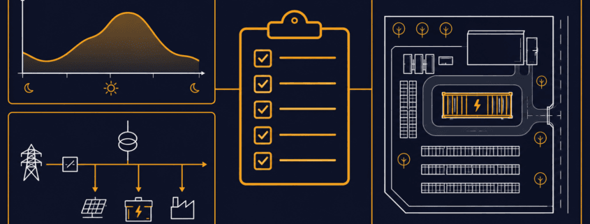
A C&I BESS quote is only as useful as the information behind it. In fact, a one-line request rarely supports reliable sizing or a comparable installed-price estimate.
Send your load data, tariff details, site facts, and main goal up front. Then every bidder answers the same question.
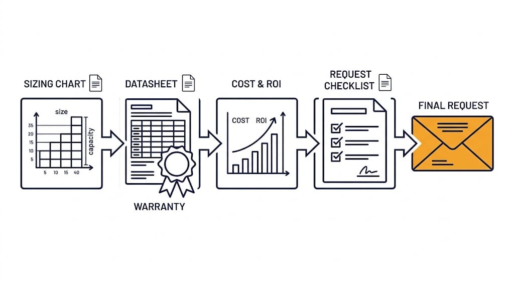
This guide covers the data, documents, and questions to prepare. Finally, it offers a request email you can copy and send.
Quick Answer: To request a C&I BESS quote, state your application, site location, target operating date, and available electrical and space details. Next, add interval load data and the tariff for savings-based projects, or critical loads and backup duration for resilience. Finally, share a single-line diagram if you have one.
Why a Generic C&I BESS Quote Is Not Enough
Asking what a 1 MWh system costs does not produce a project-ready C&I BESS quote. That is because installed cost depends on far more than battery size.
Energy duration and power rating
The application the battery must serve
Interconnection and controls
Site civil work and safety systems
Commissioning and warranty requirements
Each item changes the price. So a bare price request tells a supplier very little.
Quote preparation brings together the application, preliminary sizing, specifications, warranty requirements, and economic assumptions. However, you can refine these inputs with the supplier as the project develops.
Start Your C&I BESS Quote With the Application
Every C&I BESS quote starts with the job the battery must do. Because each job needs different data, the table below separates them.
If you have more than one goal, rank them. Otherwise, a system tuned for one job may perform poorly at another.
Prepare the Data Behind Your C&I BESS Quote
Three groups of information shape every C&I BESS quote request. Since each group answers a different supplier question, gather all three.
Energy and Tariff Information
For peak shaving and tariff-based savings analysis, aim for at least 12 consecutive months of interval data where available.
Use the utility’s demand-measurement interval, or finer data that can be aggregated to it. Also state the timestamps, time zone, units, and whether each reading is average kW or interval kWh.
Current utility bills
The full tariff or rate schedule
Demand charges, time-of-use windows, ratchets, and export compensation rules
Existing and planned solar generation data
Electrical and Site Information
Facility location and utility
Main-service voltage, transformer rating, and available capacity
Single-line diagram, where available
Existing switchgear, protection equipment, generator, and solar-inverter details
Proposed point of interconnection
Site plan, access route, usable footprint, setbacks, and fire-access constraints
Operational and Commercial Information
Main BESS use case and priority order
Target kW reduction, backup duration, or EV-charging demand
Typical operating schedule and seasonal changes
Expansion plans
Desired commercial-operation date
Budget range, procurement route, and financing preference, if you are willing to share them
Missing a document? Send what you have. Then the supplier can list the gaps and request the rest later.
What Suppliers Should Include in Their Reply
A budgetary estimate may give an indicative configuration, price range, scope, and assumptions without detailed engineering. In contrast, a developed proposal should add a more defined layout, electrical interface, commissioning scope, and itemized exclusions.
State which stage you are requesting. Also ask suppliers to flag anything that still depends on site investigation or engineering.
A strong C&I BESS quote does more than state a price. Next, ask each bidder to cover these items.
Proposed AC power rating, usable energy, and nominal energy
Stated duration at rated power
Assumed measurement boundary for capacity and efficiency
Scope of PCS, battery, BMS, EMS, HVAC, fire-safety, enclosure, and balance-of-system equipment
Interconnection and site-work assumptions
Conceptual layout and electrical-interface information, where available; more detailed drawings at the developed-proposal stage
Performance assumptions and dispatch limitations
Warranty scope, capacity retention, throughput limit, exclusions, and remedies
CAPEX breakdown, exclusions, O&M scope, and optional services
Schedule, commissioning plan, and commercial assumptions
Quote validity, currency, delivery basis, taxes or duties, payment milestones, and major price-adjustment conditions
Because unclear terms make bids hard to compare, read SunLith’s guide to understanding BESS specifications. It explains how vendors define capacity, power, and efficiency.
Also ask how the supplier plans for capacity loss over time. Our guide to BESS augmentation planning covers that topic.
Questions to Compare Across Every C&I BESS Quote
Use these questions to put every C&I BESS quote on the same footing. Ask for written answers as well, and have important assumptions, inclusions, and exclusions written into the proposal.
Capacity and Performance Questions
Is the energy rating nominal, usable DC, AC delivered, or measured at the point of interconnection?
What duration does the system provide at rated power?
Does the proposal assume one application or stacked value streams?
How are HVAC and auxiliary loads counted in efficiency and available-energy assumptions?
Scope and Ownership Questions
Which site upgrades, civil works, interconnection studies, permits, or fire-protection measures are excluded?
Who owns the EMS controls, performance monitoring, and data access?
What do commissioning, acceptance testing, training, remote monitoring, and maintenance include?
Warranty and Lifecycle Questions
Which warranty limits apply to DoD, throughput, C-rate, SOC, temperature, and dispatch?
What annual O&M and replacement costs are assumed?
What must happen for capacity augmentation, and who pays for it?
Because C-rate limits often sit inside warranty terms, see BESS C-rate explained for how those limits work.
Common Mistakes When Requesting a Quote
These errors often weaken a C&I BESS quote request. If you avoid them, your bids will be easier to compare.
Requesting price without an application: As a result, the supplier must make assumptions about the required kW, kWh, and controls.
Sharing one monthly utility bill: Because it hides peak shape, duration, and seasonal change, sizing stays uncertain.
Comparing nominal kWh with usable AC energy: Since the two numbers measure different things, the bids will not match.
Ignoring tariff and demand-charge rules: When you miss them, the value of every kW you cut is unclear.
Assuming extras are included: Unless stated, PCS, HVAC, fire protection, controls, and civil work may sit outside the price.
Comparing warranty years alone: Instead, check throughput and operating limits as well as the term.
Asking for a system sized for savings: Without sufficient load, tariff, and site information, savings-based sizing remains speculative.
Copy-and-Paste RFQ Email Template
Use this template to start your C&I BESS quote request. Replace each bracketed item with your own details before sending.
Subject: Request for preliminary C&I BESS assessment and budgetary quote
We are evaluating a battery energy storage system for [facility type] at [location]. Our primary objective is [peak shaving / backup / solar self-consumption / EV charging / other].
Attached are [interval load data / utility bills / tariff / single-line diagram / site plan].
Please provide a preliminary recommendation. Include proposed AC power, usable energy, expected duration, and key assumptions.
Also include required site or interconnection work, budgetary CAPEX, warranty summary, delivery schedule, and information needed for a detailed proposal.
Our target decision date is [date], and our target commercial-operation date is [date].
Send it to more than one supplier. Also use the same attachments each time.
Frequently Asked Questions About a C&I BESS Quote
When buyers prepare a C&I BESS quote request, the same questions come up often.
What data do I need for a C&I BESS quote?
Start with your application, site location, available electrical information, and target operating date. For peak shaving or tariff-based savings, include interval load data and the utility tariff.
For backup, provide critical-load requirements and the required backup duration. In addition, a single-line diagram and site plan help refine the proposal where available.
Can I get a C&I BESS quote with only one utility bill?
You may receive a budgetary estimate, but its sizing and savings assumptions will be limited. That is because one bill hides peak shape and seasonal change. Instead, interval data gives a far better basis.
Why do C&I BESS quotes differ so much?
Bids often use different definitions and scope. For example, one may quote nominal energy and another usable AC energy. Therefore, ask every bidder to state its assumptions.
Do I need a single-line diagram before I ask?
It helps, but it is not always required. If you lack one, send equipment nameplate details and photos of the main switchgear. As a result, the supplier can request more later.
Is a preliminary assessment the same as a final proposal?
No. A preliminary assessment gives budgetary figures and stated assumptions. However, a detailed proposal needs site-specific electrical, tariff, interconnection, and safety review.
Ready to Request a Preliminary Assessment?
Contact SunLith for a C&I BESS quote with your project objective, site location, and available load, tariff, and electrical information. If documents are missing, explain what you have so we can identify the next steps.
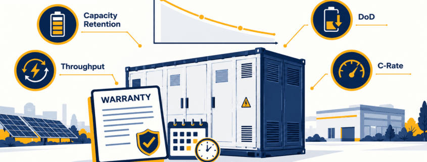
A C&I BESS warranty is not just a number of years. It is a contract that guarantees performance only inside a defined operating envelope.
That envelope covers capacity, throughput, depth of discharge, C-rate, and temperature. However, operating outside a stated limit may reduce coverage or affect a claim, depending on the contract terms and the documented cause of the issue.
First, this guide shows how to read each term before you sign. It also ties the warranty back to your peak-shaving BESS sizing, so the system can still meet your kW and kWh needs late in life.
⚡ Quick Answer: A C&I BESS warranty is more than a number of years. It is a set of performance promises that apply only within defined operating limits. So check guaranteed capacity, throughput, depth of discharge, C-rate, temperature, test method, exclusions, and the remedy before you compare suppliers.
What a C&I BESS Warranty Actually Covers
A C&I BESS warranty usually bundles several separate promises. Scope, duration, and exclusions vary by supplier and contract, so read each promise on its own.
Product or defect warranty: covers faulty parts and manufacturing defects.
Capacity-retention warranty: guarantees a minimum state of health (SoH) at set points in time.
Throughput or cycle-life warranty: limits the total energy or cycles the system may process.
Performance warranty: may add an efficiency commitment, depending on the contract.
Workmanship warranty: covers installation quality when SunLith or an EPC provider supplies it.
Subsystem coverage: identifies whether the PCS, EMS, BMS, HVAC, enclosure systems, and any supplied fire-detection or suppression equipment are covered, and for how long.
Also, each item can carry its own term, limits, and remedy. For example, a long cell warranty does not prove the PCS or cooling system is covered for as long.
C&I BESS Warranty Terms: Capacity Retention vs. Throughput
Most disputes over a C&I BESS warranty start with two terms. But capacity retention and throughput control very different things.
Term
What it controls
Buyer question
Capacity retention / SoH
Remaining usable energy at a specified point in time
At what measurement boundary and operating conditions is capacity tested?
Throughput
Total permitted energy processed during the warranty
Is throughput counted one way, both ways, or as equivalent full cycles?
Equivalent full cycles
An accounting measure of throughput relative to capacity
What capacity denominator and counting method does the contract use?
End-of-life threshold
The contractual capacity floor at a stated year or throughput value
Does that floor still satisfy the project’s service obligation?
Capacity Retention and State of Health
Capacity retention sets the minimum usable energy at a stated point in time. For example, a contract might guarantee 70% of baseline capacity at year 10 (illustration only).
First, the key issue is the measurement boundary. Capacity can be quoted at the cell, the DC bus, the PCS AC output, or the point of interconnection.
Because of this, each boundary gives a different number. Also confirm the beginning-of-life baseline, because a retention percentage means little without it.
Throughput and Equivalent Full Cycles
A throughput provision may limit the cumulative energy processed during the warranty. For example, some contracts count discharge only, while others count charge and discharge together.
Then equivalent full cycles convert that energy into a cycle count. The result depends on the capacity used as the denominator, so ask for the exact formula.
An open-access review in Energies discusses degradation models based on cumulative energy throughput. It also covers models that account for cycling conditions such as depth of discharge, state of charge, and temperature.
But contracts often use the simpler count. Your dispatch pattern still decides how fast the cells age, so learn how equivalent full cycles and throughput records are tracked in the BMS.
End-of-Life Thresholds
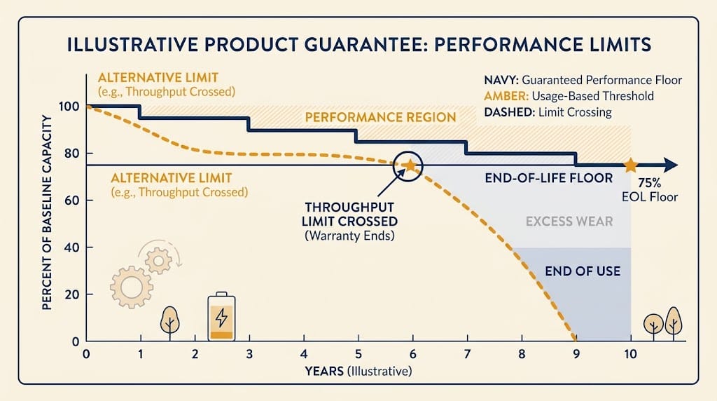
An end-of-life threshold is the contractual capacity floor a supplier agrees to support, subject to the stated terms. It applies at the year or throughput value that the contract names.
Then check that this floor still meets your service obligation. As a result, a battery can meet its warranty floor and still miss your load requirement.
Capacity fades on two clocks, time and use. See calendar and cycle aging for how each one works.
The Operating Envelope Behind Every C&I BESS Warranty
Every C&I BESS warranty rests on assumed operating conditions. As a result, if the site operates outside those conditions, coverage may be limited or a claim may be disputed under the contract.
A warranty can be technically valid but commercially unsuitable if the operating limits do not match the intended dispatch plan.
Charge, Discharge, and Depth Limits
First, list every electrical limit the contract sets. Typical items include:
Maximum and minimum state of charge
Permitted depth of discharge
Charge and discharge C-rate
Throughput terms often carry a maximum C-rate clause as well. Then compare your peak discharge power against the BESS C-rate limit in the contract.
Time, Temperature, and Throughput Limits
Next, check the limits tied to time and environment:
Temperature and humidity requirements
Calendar limits versus cycling limits
Annual or cumulative throughput limits
For example, many contracts specify that coverage ends when the first applicable limit is reached. So look for the phrase “whichever occurs first.”
Controls, Data, and Maintenance Duties
Finally, review what the owner must do to keep coverage intact:
Follow the approved EMS settings and dispatch behavior
Complete the required maintenance
Keep connectivity, monitoring, and event logging active
However, missing data can make a claim hard to win. Our guide to evaluating a supplier’s BMS also explains SOH and throughput logging.
Sizing sets your first kW and kWh requirement. The C&I BESS warranty then decides whether the system can keep meeting it.
Take the 100 kW / 278 kWh preliminary configuration in the peak-shaving guide. It illustrates how first-year power and energy requirements can be estimated for one defined peak event.
However, whether it can meet repeated events or retain enough capacity late in life depends on the operating plan and the warranty’s limits.
Next, here is a simple, hypothetical check. If a contract permits 3,000 equivalent full cycles, and the site uses one equivalent full cycle on each day it operates, daily cycling would reach that limit in about 8.2 years (3,000 ÷ 365).
But if the system uses one equivalent full cycle on only 150 days each year, it would take about 20 years to reach the same limit. Calendar limits may then determine when coverage ends.
Also, an equivalent full cycle is an energy measure, not a single dispatch event. These figures are illustrations, not market terms.
So check size and dispatch strategy against the warranted envelope, not just first-year savings. Warranty terms also feed your BESS OPEX and CAPEX vs LCOS assumptions, because lost throughput raises the cost of each delivered kWh.
C&I BESS Warranty Checklist for RFQs
First, use this C&I BESS warranty checklist in every request for quotation. Ask each supplier the same questions so the answers compare cleanly.
Capacity and Baseline Questions
Is capacity measured as nameplate, usable DC, PCS AC, or energy at the point of interconnection?
Which beginning-of-life capacity baseline applies?
How much retained capacity is guaranteed at each year or throughput checkpoint?
Which testing method verifies capacity, and under what site conditions?
Throughput and Operating Limit Questions
Is there a calendar limit, cycle limit, throughput limit, or a “whichever occurs first” condition?
How is throughput counted: charging, discharging, both directions, or equivalent full cycles?
What DoD, C-rate, temperature, SOC range, and dispatch pattern does the warranty assume?
How is an equivalent full cycle calculated and logged?
Scope, Exclusion, and Remedy Questions
Which components are included: cells, modules, racks, BMS, PCS, HVAC, EMS, enclosure systems, and any supplied fire-detection or suppression equipment?
Which exclusions can reduce or invalidate coverage?
What data must the owner retain to support a claim?
If the system misses a warranted value, what is the remedy: repair, replacement, payment, capacity augmentation, or another remedy? Who pays for labor, logistics, downtime, testing, and recommissioning?
Since the remedy may be added capacity, plan that work early. Our guide to BESS augmentation planning explains how lost capacity is restored.
Common Mistakes When Comparing Warranty Bids
Buyers often repeat the same errors when they compare bids. Next, avoid these five:
Comparing years alone: two bids with equal terms can carry very different limits.
Ignoring the measurement boundary: a DC figure and an AC figure are not the same promise.
Assuming equal throughput counting: one bid may count discharge only, another both directions.
Skipping the dispatch check: the warranty may not fit your real duty cycle.
Accepting a vague remedy: insist on clear timing, cost, and responsibility.
Frequently Asked Questions About a C&I BESS Warranty
These answers cover the questions buyers ask most about a C&I BESS warranty.
What does a C&I BESS warranty cover?
It usually covers defects, a capacity or state-of-health guarantee, and sometimes a throughput limit. Also, scope and duration vary by supplier and contract.
How do capacity retention and throughput differ?
Capacity retention sets a minimum usable energy at a point in time. Meanwhile, throughput caps the total energy the system may process during the warranty.
Can a C&I BESS warranty be valid but still unsuitable?
Yes, because if its limits on depth, C-rate, or throughput do not match your dispatch plan, the system can reach a contract limit early.
What is a BESS performance warranty?
A BESS performance warranty defines measurable commitments, such as usable capacity, capacity retention, energy throughput, availability, or efficiency, under specified test conditions and operating limits. The exact scope and remedy depend on the contract.
What is end of life in a BESS warranty?
It is the contractual capacity floor at a stated year or throughput value. Then confirm that it still covers your required kWh.
Who should review a BESS warranty before signing?
Your engineer, procurement lead, and legal counsel should each review it. SunLith can provide a preliminary specification review, but contract terms need qualified legal review.
Need a Preliminary Warranty Review?
Send us your datasheet and draft warranty terms. Then we will flag the limits that matter for your dispatch plan.
SunLith can provide a preliminary assessment. Final system design and contract terms require site-specific electrical, tariff, interconnection, safety, and legal review.
Further Reading on the C&I BESS Warranty and Related Costs
Also, use these guides alongside this C&I BESS warranty guide.
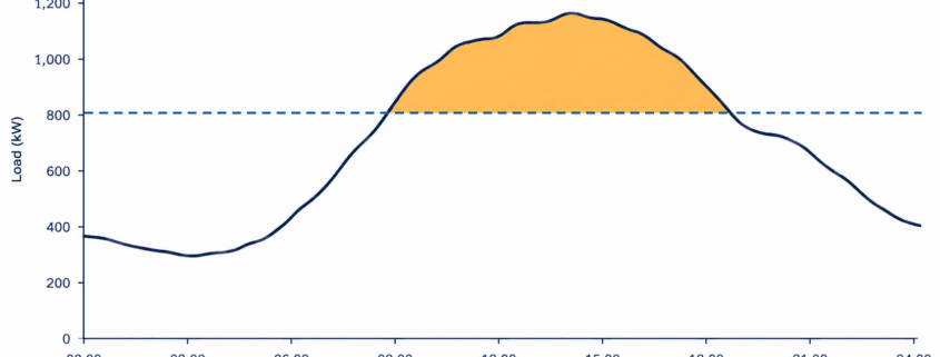
Peak shaving battery sizing starts with two questions. How much power must the battery discharge? For how long? First, choose the maximum grid demand you want your facility to draw. Then analyze your interval load data. The highest load above that target sets the discharge power, in kW. The area above the target sets the delivered energy, in kWh.
Quick Answer
Peak-shaving battery sizing starts by subtracting the selected grid-demand target from site load in each interval. The highest result is the preliminary battery discharge-power requirement in kW. Add the interval discharge energy to estimate delivered kWh, then adjust for defined discharge efficiency and permitted usable capacity.
Those two numbers are only a starting point, though. A workable design must also account for discharge losses and the battery’s allowed operating range. It also needs to handle repeated peaks, charging opportunities, and how your utility calculates billed demand. Peak shaving means discharging a battery to cut peak grid demand. That is different from shifting energy use to another time, or sizing a battery for outage backup.
The Peak Shaving Battery Sizing Formulas at a Glance
Peak shaving battery sizing follows four simple steps for each interval in your load data. Confirm the measurement boundary, such as battery DC terminals, PCS AC output, or site meter, before applying efficiency assumptions.
New to these units? SunLith’s Ah vs Wh battery capacity guide covers the Wh = Ah × voltage relationship behind every kWh figure below.
Key Sizing Formulas
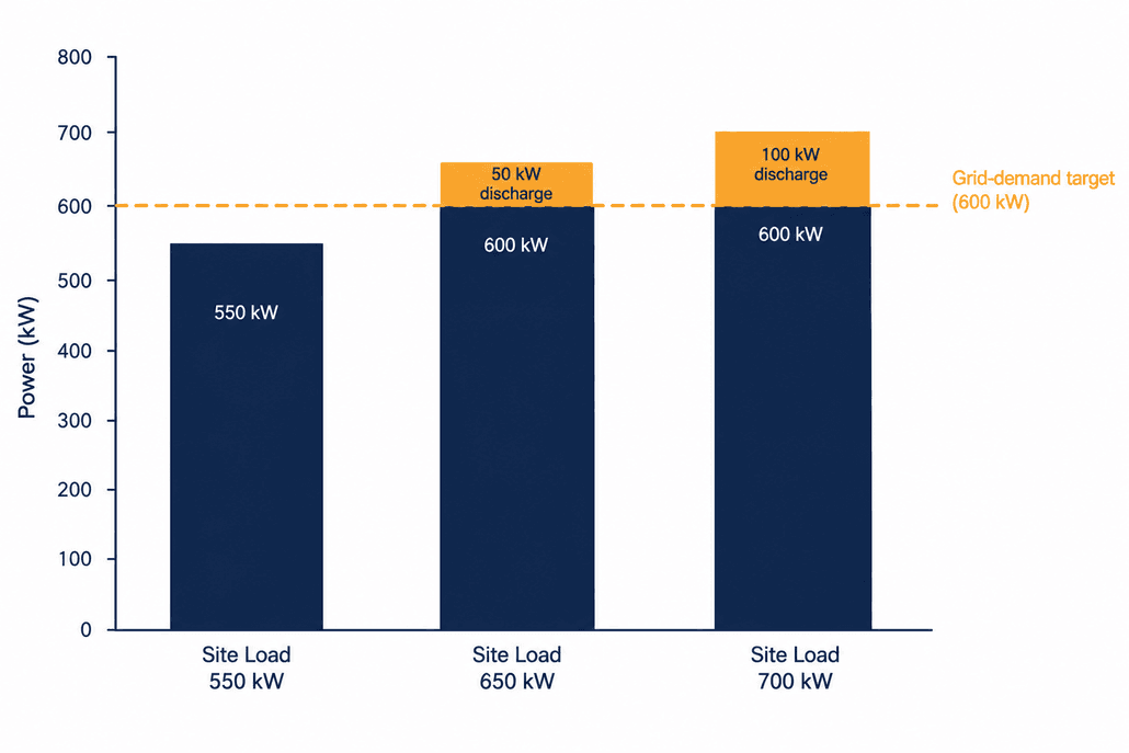
First, find the battery discharge required, in kW. Take site load, subtract the grid-demand target, and floor the result at zero. A 700 kW load against a 600 kW target needs 100 kW of discharge. A 550 kW load against the same target needs none.
Pbattery,i = max(0, Li − T)
Next, find the largest required discharge across every interval. That becomes your preliminary AC discharge-power requirement.
Prequired = maxi(Pbattery,i)
Then find the delivered energy, in kWh. Add up, across every interval in one peak event, the discharge required multiplied by the interval length in hours.
Edelivered = Σi(Pbattery,i × Δti)
Finally, estimate nominal battery capacity. Divide delivered energy by discharge efficiency, then by the usable fraction of nominal capacity. Discharge efficiency is the assumed efficiency from the battery’s energy boundary to the AC delivery point. The usable fraction is the share of nominal capacity available for this duty. Define both terms before you apply the formula, since this is only an event-level estimate. It is not a substitute for simulating state of charge over time.
Enominal = Edelivered ÷
(ηdischarge × fusable)
Where: Pbattery,i is the required battery discharge during interval i;
Li is site load; T is the selected grid-demand target;
Δti is interval duration in hours;
ηdischarge is defined one-way discharge-path efficiency; and
fusable is the permitted usable share of nominal capacity.
Step 1: Gather Load Data and the Tariff
First, ask your utility or metering provider for interval demand data covering representative operations and seasons. You need to see the shape of each peak, not just the highest number on a bill. A 100 kW exceedance lasting 15 minutes requires far less delivered energy than the same exceedance lasting three hours.
Also collect the tariff alongside the data. Identify the demand-measurement interval. Check which periods carry demand charges. Look for other billing provisions that affect the value of reducing a peak. The target should be based on how demand is measured and billed under the applicable tariff, not a generic assumption about demand charges.
One MDPI-published study of low-voltage commercial users evaluated battery energy capacity against measured customer-load data and the resulting peak reduction over time. The principle for a single facility is the same: use interval data rather than a monthly peak alone.
If the site has solar, use net demand at the relevant meter. Also model how solar output varies during likely peak events. A sunny-day profile alone may understate the battery needed on a cloudy day.
Step 2: Choose a Grid-Demand Target
Suppose a facility’s load sometimes reaches 700 kW. You could test targets of 650 kW, 600 kW, and 550 kW. Generally, a lower target asks the battery to provide more power, more energy, or both. However, whether that extra capacity pays off depends on the tariff and the full pattern of peaks.
Do not pick the target from the single highest reading alone. A battery might shave the largest peak successfully. Then it may exhaust its usable energy during a longer, lower peak later that day.
Step 3: Calculate Required Battery Power
For each interval, subtract the target from site load. If the result is negative, set the discharge requirement to zero. The table below shows this for a 600 kW target.
Example: discharge needed to hold a 600 kW target
Site load
Discharge needed to hold 600 kW
550 kW
0 kW
650 kW
50 kW
700 kW
100 kW
The preliminary requirement here is 100 kW of AC discharge power, measured at the point where the battery offsets meter demand. An engineer must then confirm that the chosen power conversion system and installation can sustain that output under real operating conditions.
Step 4: Calculate the Delivered Energy for Each Peak
Power tells you how fast the battery must discharge, while energy tells you how much it must deliver over the whole event.
For preliminary analysis, define a peak event as consecutive metering intervals where site demand stays above the selected grid-demand target. If demand drops below the target and the battery can begin recharging, treat the next exceedance as a separate event. Verify that the available recharge time and charging-power limit are sufficient.
Assume the facility stays at 700 kW for one hour. Then it drops to 650 kW for two hours, still against a 600 kW target. That gives 100 kW for one hour, plus 50 kW for two hours. The total is 200 kWh delivered.
So this event requires 100 kW of maximum discharge and 200 kWh of delivered AC energy. A battery rated for 100 kW but able to deliver only 100 kWh would not cover the whole event at this target.
Repeat this calculation for other days and seasons. The event with the highest instantaneous discharge sets one constraint. The event with the greatest delivered energy may set the energy-capacity requirement.
Step 5: Estimate Nominal Battery Capacity
The battery must store more energy than it ultimately delivers. Discharge is not lossless, and the full nominal capacity may not be available for the chosen operating strategy.
For illustration, assume 200 kWh of required delivered energy. Assume a 90% one-way discharge-path efficiency and an 80% permitted usable fraction of nominal capacity. Divide 200 by 0.90, then by 0.80. That gives roughly 278 kWh of nominal capacity.
That figure is only an initial estimate, not a recommended product size. First, check the vendor’s capacity definition. Then account for state-of-charge limits, expected end-of-life capacity, temperature effects, auxiliary consumption, warranty commitments, and the manufacturer’s defined AC or DC capacity boundary before choosing a product.
Accounting for Discharge Losses vs. Round-Trip Efficiency
Do not treat round-trip efficiency as one-way discharge efficiency. Round-trip efficiency includes losses across both charging and discharging. Applying it as a discharge factor, then adding separate discharge losses on top, counts losses twice. A preliminary sizing tool may use round-trip efficiency as a simplified assumption. Final peak shaving battery sizing should still call out discharge-path losses on their own.
SunLith’s guide to understanding BESS specifications explains how vendors actually define usable capacity and efficiency, both needed for this step.
Step 6: Test Repeated Peaks and Recharging
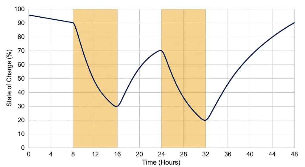
The example above assumes the battery has enough charge when the event begins. Real facilities may see several peaks a day, peaks on consecutive days, or an unusually long stretch above the target. Charging too aggressively can itself create a new metered peak.
Run the load profile forward, interval by interval, using these five steps.
Begin with an assumed battery state of charge.
Discharge whenever load would otherwise exceed the chosen target.
Track remaining energy and all applicable losses.
Allow charging only when it fits the tariff, site load, and equipment limits.
Check whether the battery is ready for the next event.
This simulation may reveal that a seemingly adequate 100 kW / 278 kWh preliminary configuration needs more capacity. Or it may show that a different demand target produces a better project. Model peak-shaving dispatch and resulting bill impacts together this way, instead of inferring them from a single peak value.
Sample Interval-Data Worksheet Columns
A simple spreadsheet makes this simulation easier to run and easier to hand to an engineer. Track these six columns for every interval in the load dataset.
Column
What it records
Timestamp
Date and interval start time
Site load (kW)
Measured or forecast demand for the interval
Target (kW)
The grid-demand target being tested
Discharge required (kW)
Site load minus target, floored at zero
Delivered energy (kWh)
Discharge required times interval hours
Simulated state of charge (%)
Running battery charge after each interval
Step 7: Check Whether the Battery Size Makes Financial Sense
A technically workable target is not always the most economical one, though. Compare several combinations of battery power, energy, and target demand against the real tariff and a no-storage baseline. Include the cost of charging, equipment and installation, operating costs, and expected capacity changes over the project life.
SunLith’s peak shaving vs load shifting guide explains the two strategies and where they overlap. Use it to understand the value stream, not as an interval-based sizing tool.
For the financial modeling itself, SunLith’s guide to calculating BESS ROI walks through the cash-flow side. Use it once the power and energy numbers from this sizing exercise are in hand.
Common Peak Shaving Battery Sizing Mistakes
Because these errors repeat across projects, they turn a sound peak shaving battery sizing exercise into an undersized or overpriced one.
Using only the monthly peak: It does not show how long or how often demand exceeds your target.
Confusing kW with kWh: The maximum exceedance sets discharge power. Duration and shape set delivered energy.
Sizing from one favorable day: Solar production, weather, occupancy, and operations can all change the peak profile.
Ignoring the next event: The battery may suit one peak but fail to recharge before another.
Assuming every kWh of nameplate capacity is usable: Operating limits and performance requirements must be checked against the proposed product.
Treating demand-charge savings as guaranteed: Actual savings depend on successful dispatch and the applicable tariff.
Frequently Asked Questions About Peak Shaving Battery Sizing
These questions come up often once a facility starts peak shaving battery sizing from its own interval data.
Can I size a peak shaving battery from a utility bill?
A bill shows billed demand and charges, but it usually will not show the full duration and shape of the peaks. First, use interval data for a credible power-and-energy estimate. Then apply the tariff to evaluate savings.
Is a 100 kW battery enough to reduce my peak by 100 kW?
Not necessarily. First, it must deliver that power at the relevant point in the electrical system. Also, it needs enough energy and state of charge for the whole event. Finally, it must stay available for other peaks that affect the bill.
How many hours of battery storage do I need for peak shaving?
There is no universal duration. First, calculate the energy above your chosen demand target across actual events. Then test whether the proposed power and energy ratings can meet those events repeatedly.
Is peak shaving battery sizing the same as backup sizing?
No. Peak shaving battery sizing follows measured site demand above a grid-import target. Backup sizing starts instead with the critical loads that must run during an outage, and the required backup duration. It is a different starting point and a different formula set. For preliminary outage-backup estimates, use SunLith’s C&I BESS sizing calculator. It uses critical-load and backup-duration inputs, so it should not be used to size a peak-shaving system.
This article gives a preliminary sizing method, not an equipment specification or a savings guarantee. Final selection still needs interval-data and tariff analysis, electrical design, and product-specific validation.
Need a Peak-Shaving BESS Assessment?
A preliminary battery size should be tested against your actual interval demand data, tariff rules, charging windows, and operating priorities. Send SunLith your site load profile and utility tariff for an initial C&I BESS assessment.
A C&I BESS sizing calculator answers one question fast. How big should the battery and inverter be?
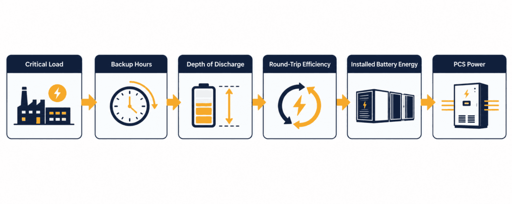
It turns your critical load and backup hours into two numbers. First, installed battery energy in kWh. Second, PCS power in kW.
Use the free calculator below for a preliminary estimate. Then review the formulas, assumptions, and worked example before making project decisions.
Quick Answer: A C&I BESS sizing calculator turns your critical load and backup hours into two numbers. Installed battery energy in kWh factors in depth of discharge and round-trip efficiency. PCS power in kW adds a safety margin to your critical load. Still, this is a preliminary size, not a final design.
Try the C&I BESS Sizing Calculator
This calculator runs instantly in your browser. Once you enter a few numbers, it returns a preliminary size.
Enter your peak site load, critical load, and backup duration below. Then adjust depth of discharge, round-trip efficiency, and reserve margin if you have better numbers than the defaults.
C&I BESS Sizing Calculator
Estimate preliminary BESS power (kW/MW), installed battery energy (kWh/MWh), usable capacity, and backup duration.
Checks that critical load is realistic. It does not set PCS size unless whole-site backup is required.
Load that must operate during an outage.
Preliminary assumption. Final design should use discharge-path losses and auxiliary loads.
Advanced assumptions
Your preliminary C&I BESS size
Recommended BESS power—
Installed battery energy—
Estimated usable capacity—
Minimum apparent rating—
Target backup duration—
Nominal E/P duration—
Estimated required C-rate—
Installed battery energy is the nominal battery capacity required after DoD, simplified system efficiency, and reserve margin, not the nameplate size on its own.
This is a preliminary estimate. Final BESS sizing requires interval-load analysis, electrical design, site conditions, grid requirements, safety review, and product-specific warranty validation.
The results show recommended PCS power and installed battery energy. They also show usable capacity, minimum apparent power, and the required C-rate.
It works on desktop and mobile browsers alike, with no signup and no limit on how many times you recalculate.
Preliminary sizing only. This calculator estimates battery energy and PCS power from the inputs you provide. It is not a final design, quotation, or performance guarantee. It also does not replace an interconnection study, fire-safety review, or full interval-load analysis.
Why C&I BESS Sizing Matters for Commercial and Industrial Sites
Demand charges and outage risk both push sites toward battery storage. So a C&I BESS sizing calculator earns its place from the first estimate.
But get the size wrong, and the cost shows up either way.
Demand charges can be steep. In fact, research from the National Renewable Energy Laboratory (NREL), cited in this NYSERDA research summary, puts them at 30 to 70 percent of a typical commercial bill.
For example, an undersized battery cannot cover the critical load for the full outage. An oversized one, meanwhile, ties up capital that could fund other work.
A sizing calculator will not replace formal engineering design. But it still gives you a fast, defensible starting point.
Many C&I storage decisions, in turn, weigh demand-charge savings alongside backup value, though actual payback varies widely by project, utility rate structure, and site load profile.
What This C&I BESS Sizing Calculator Estimates
This calculator has one job: outage backup. Enter a critical load and a backup duration. Then it returns a preliminary size.
It is not a peak-shaving calculator. Instead, peak shaving needs interval load data and your utility’s demand-charge structure, not just a critical load.
Cutting demand charges is a different goal. See our guide to C&I BESS peak shaving instead.
Facility managers, EPCs, and asset owners typically use this stage of sizing before requesting formal quotes from vendors.
How to Find Your C&I BESS Sizing Calculator Inputs
Most sizing mistakes start with the inputs, not the formulas. Get these right first, and the C&I BESS sizing calculator results are far more reliable. Rough numbers are fine at this stage; precise numbers can wait for the engineering phase.
Critical load: list every circuit that must run through an outage. Think life-safety systems, refrigeration, servers, security, and any process equipment that cannot tolerate downtime. Then sum their running kW, not nameplate or inrush kW.
Peak site load: pull this from 12 months of utility interval data if you have it. Otherwise, use your utility bill’s peak demand figure as a starting point.
Backup duration: match this to your actual outage risk, not a round number. A site with frequent short outages needs a different duration than one preparing for extended grid events, so review recent outage history if it exists.
Site documentation, meanwhile, helps too. Single-line diagrams, panel schedules, and recent utility bills all help validate your critical-load list before you finalise it.
Power factor and reserve margin, by contrast, are usually starting assumptions rather than measured figures. Adjust them once your battery vendor or EPC confirms real numbers.
The Sizing Formulas Behind the Calculator
Every result from this C&I BESS sizing calculator comes from one of the formulas below. Here is what each one does, and why it matters.
Delivered Backup Energy
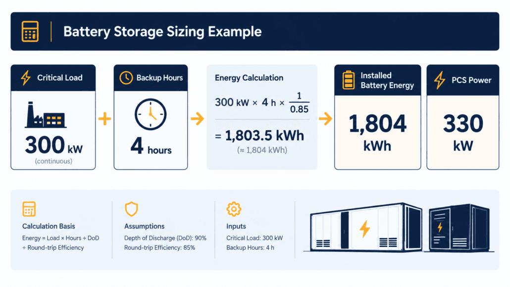
Delivered backup energy is critical load multiplied by backup hours. A 300 kW critical load for four hours, for example, needs 1,200 kWh delivered.
In short, this is the energy your equipment actually uses. It is not yet the battery size, since no battery discharges every stored kWh.
A facility with several critical circuits should sum them before running this figure.
Installed Battery Energy
Installed battery energy has three steps. First, divide delivered energy by depth of discharge. Then divide again by round-trip efficiency. Finally, add a reserve margin.
Together, DoD and RTE shrink how much nameplate capacity you can actually use. The reserve margin, meanwhile, covers degradation, temperature, and load uncertainty.
Most C&I LFP batteries run 85 to 95 percent depth of discharge. Round-trip efficiency usually sits between 90 and 95 percent at the system level. Always confirm this with your manufacturer’s datasheet.
Round-trip efficiency is a simplified, conservative assumption for a preliminary calculator. Final backup sizing should instead use discharge-path efficiency. That includes PCS, transformer, cable, battery, and auxiliary-load losses at the actual operating condition.
A wider site temperature range usually pushes real-world RTE toward the lower end of that band.
Recommended PCS Power and Apparent Power
Similarly, recommended PCS power is critical load times one plus a power margin. A 10 percent margin is a preliminary allowance only, and motor starting or other transient loads still need separate review.
Minimum apparent power in kVA, meanwhile, divides that PCS power by your system power factor. This is the screening figure for PCS and transformer ratings.
A lower power factor raises the apparent-power requirement, which can affect transformer selection.
C-Rate and Nominal E/P Duration
Finally, required C-rate is PCS power divided by installed battery energy. It shows how hard you are asking the battery to discharge.
Nominal E/P duration, by contrast, is installed battery energy divided by PCS power. Watch this figure closely. It often differs from your target backup hours, since DoD, RTE, and reserve margin all pull it away from a clean match.
A lower target C-rate generally means a larger, more conservative battery for the same PCS power.
Calculation
Formula
Meaning
Delivered backup energy (kWh)
Critical load (kW) × backup duration (hours)
Energy the critical load needs during the outage.
Installed battery energy (kWh)
(Delivered ÷ (DoD × RTE)) × (1 + reserve margin)
Nominal capacity required after DoD, system efficiency, and reserve margin.
Usable battery capacity (kWh)
Installed battery energy × DoD
Energy within the chosen discharge window.
Recommended PCS power (kW)
Critical load × (1 + power margin)
Suggested continuous PCS output rating.
Minimum apparent power (kVA)
Recommended PCS power ÷ power factor
Screening value for PCS and transformer rating.
Required C-rate
Recommended PCS power ÷ installed battery energy
Power-to-energy relationship indicator.
Nominal E/P duration (hours)
Installed battery energy ÷ recommended PCS power
Configuration indicator, not a runtime guarantee.
A C&I BESS Sizing Calculator Worked Example: 300 kW Critical Load
This worked example uses an 800 kW peak load and a 300 kW critical load. Backup duration is four hours.
Assumptions: 85% depth of discharge, 90% round-trip efficiency, 15% reserve margin. Also: 10% power margin, 0.90 power factor.
Nominal E/P duration: 1,804 ÷ 330 = 5.5 hours. That’s longer than the 4-hour target. DoD, RTE, and reserve margin together explain the gap.
This C&I BESS sizing calculator worked example uses one input combination. Change the backup duration to 2 hours, and installed battery energy roughly halves.
Push reserve margin to 20 percent instead, and it grows a little further. Run a few combinations of your own before settling on a target range.
Common C&I BESS Sizing Calculator Mistakes
These mistakes show up again and again in early estimates. But each one is easy to avoid once you know to check for it, and most take only a few extra minutes to correct before you share a number with anyone.
Ignoring DoD and RTE. In practice, sizing straight off delivered energy leaves a battery that cannot actually deliver the promised backup.
Skipping the reserve margin. Batteries lose usable capacity over time. A 10 to 15 percent margin, therefore, buys headroom for later years, not just day one.
Confusing power and energy. In short, a 330 kW PCS and a 1,804 kWh battery answer two different questions. Size both instead of just one.
Ignoring the required C-rate. For instance, a high C-rate can raise thermal stress and cut usable capacity under load. It can also affect cycle life and fall outside warranty limits. Confirm your chosen battery and PCS support the required rate.
Skipping fire code and siting review. NFPA 855, local fire and building codes, the authority having jurisdiction, and UL 9540A test evidence can all affect separation distances and layout. A preliminary estimate still needs a compliant site review. See our NFPA 855 guide for more detail.
Using nameplate load instead of running load. Nameplate and measured running load serve different purposes. Size the C&I BESS sizing calculator energy inputs off measured running kW, but review starting and transient loads separately for PCS sizing.
Skipping a sensitivity check. Run the calculator twice: once with conservative assumptions, once with optimistic ones. The gap between the two shows how much margin your estimate really has.
When You Need More Than a C&I BESS Sizing Calculator
Peak shaving, tariff optimisation, solar shifting, and generator integration all need more than one critical-load input. So do data centres and microgrids.
Peak shaving needs interval load data and your target demand level. Our demand charge guide covers why that line item is often 30 to 70 percent of a commercial bill.
Treat this calculator’s output as a starting point instead. Overall, bring it to an engineer, not to a procurement order.
Solar-plus-storage sizing is another case this C&I BESS sizing calculator does not cover. A hybrid system needs production profiles, self-consumption targets, and export limits alongside backup requirements.
Multi-building campuses work differently too. Size each building’s critical load separately, then combine the installed-energy totals rather than averaging duration targets across buildings.
Frequently Asked Questions
Quick answers to the most common C&I BESS sizing calculator questions, covering inputs, assumptions, and accuracy.
What inputs does a C&I BESS sizing calculator need?
At minimum: peak site load, critical load, and backup duration. Depth of discharge, round-trip efficiency, reserve margin, power margin, and power factor refine the estimate further.
What depth of discharge and round-trip efficiency should I use for LFP?
Most C&I LFP systems run 85 to 95 percent usable depth of discharge. Round-trip efficiency is usually 90 to 95 percent at the system level. Still, confirm exact figures with your manufacturer’s datasheet.
How much reserve margin should I add?
10 to 15 percent is a common starting point. It covers degradation, temperature swings, and load uncertainty. Still, longer contracts or harsher climates justify a larger margin.
Is a C&I BESS sizing calculator accurate enough for procurement?
No. Treat it as a preliminary estimate instead. Final sizing needs interval-load analysis, electrical design, site conditions, grid requirements, and product-specific warranty terms.
What’s the difference between installed and usable battery capacity?
Specifically, installed capacity is the nominal or nameplate energy capacity selected for the system. It is sized above the delivered-load requirement to account for DoD, system efficiency, and reserve margin. Usable capacity, by contrast, is the portion available within the selected DoD window.
Can this calculator size a multi-building campus?
Not directly in one pass. Run it once per building using each building’s own critical load and backup duration, then combine the installed-energy results before selecting a shared BESS.
How often should I re-run the calculator during a project?
Re-run it whenever a key input changes, such as an updated critical-load list, a revised backup target, or new DoD and RTE figures from a vendor quote. Treat early results as a starting range, not a fixed number.
Does this calculator account for battery degradation over time?
The calculator does not explicitly model year-by-year degradation. Its reserve margin is a user-selected allowance, not a validated end-of-life guarantee. Actual fade depends on chemistry, duty cycle, temperature, and your warranty terms.
Further Reading
More Sunlith guides pair well with this C&I BESS sizing calculator, covering fire code compliance, demand charges, and cost planning for C&I storage projects generally.
Disclaimer: This calculator and article provide preliminary estimates only. Final BESS sizing requires interval-load analysis, electrical engineering design, site assessment, applicable grid and fire codes, and manufacturer-specific validation.
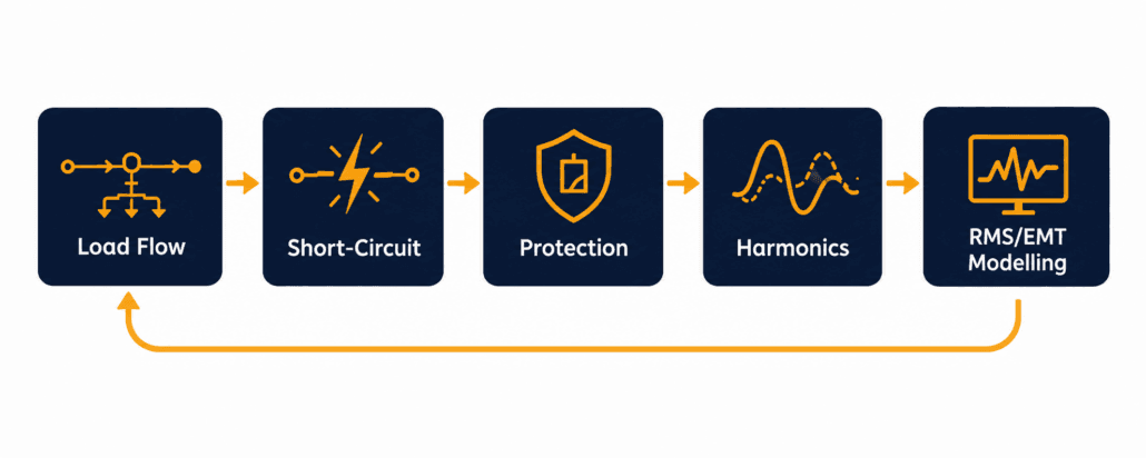
BESS grid connection studies are the engineering checks a network operator runs before it approves a battery storage project. Each study asks the same underlying question: can this plant connect and operate without exceeding voltage, thermal, fault-level, protection, or power-quality limits at the connection point? This guide covers the core BESS grid connection studies: load flow, short-circuit, protection coordination, harmonics, and RMS/EMT dynamic modelling.
Last reviewed: September 2026. Study requirements vary by network operator, project design, grid strength, and applicable grid code.
This guide walks through:
What each of the core study types actually checks
Why RMS and EMT modelling are different tools, not two names for the same thing
Where these studies sit inside the wider interconnection timeline
What a BESS developer needs to supply before a network operator can run them
Common reasons a study package gets rejected or delayed
Quick Answer
BESS grid connection studies are the technical checks a network operator runs before interconnection: load flow, short-circuit, harmonics, and RMS/EMT dynamic modelling. Together, they confirm a battery project can connect safely, without degrading voltage, fault protection, or power quality on the connecting network.
BESS Grid Connection Studies Checklist
Before locking the BESS configuration or signing a PCS supply agreement, work through this checklist.
Identify the likely point of connection, voltage level, and export/import capacity
Obtain the network operator’s formal study scope, model format, and submission timeline
Confirm whether the plant must operate grid-following, grid-forming, or both
Obtain validated RMS models, and EMT models where required, for the PCS and plant controller
Confirm the model’s operating range, control modes, fault-response logic, and firmware version
Screen local grid strength, nearby inverter-based resources, and background harmonic levels early
Reserve schedule time for model review, study reruns, and compliance testing
Carry a contingency for mitigation measures such as filtering, a revised export limit, or grid-forming controls
What Are BESS Grid Connection Studies?
BESS grid connection studies answer one question. Can this project connect here safely? The network operator studies the plant at its point of interconnection (POI), sometimes called the point of common coupling (PCC). It then compares the results against the planning limits already set for that part of the grid.
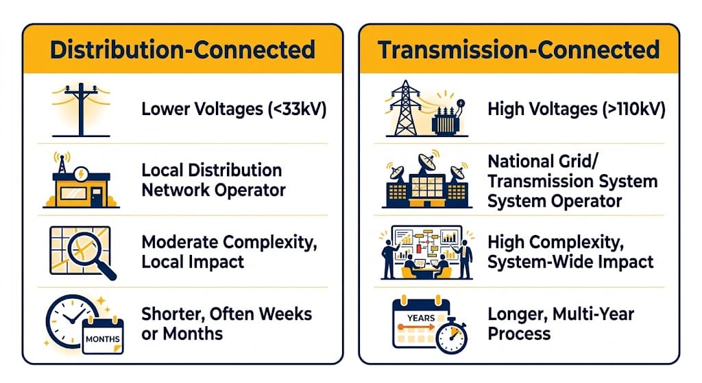
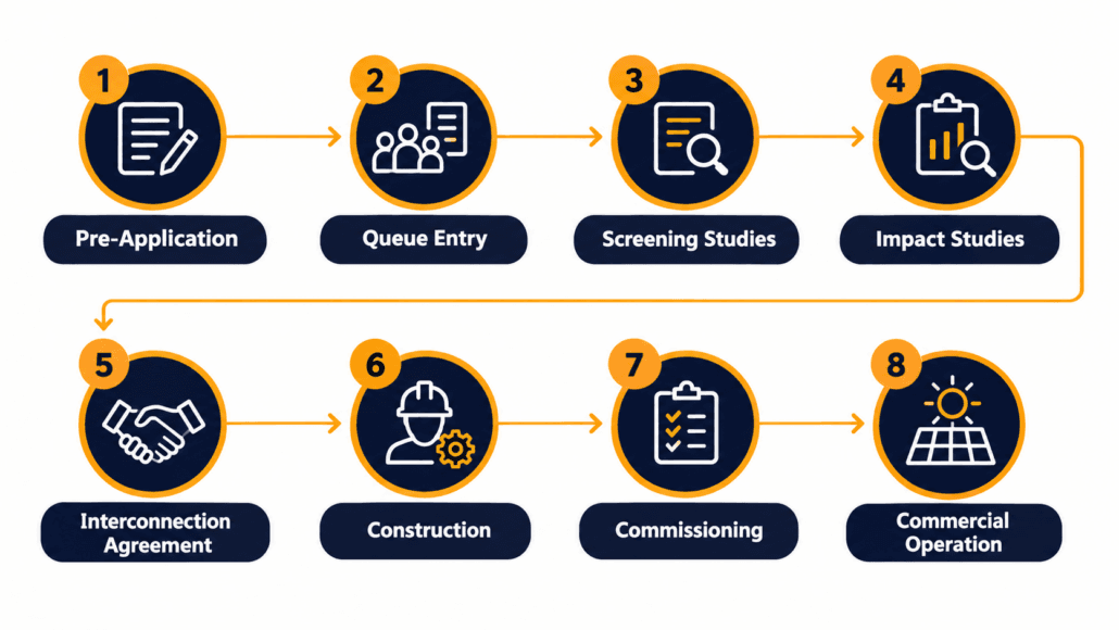
Specifically, study scope depends on three main factors: project size, connection voltage, and how electrically “stiff” or “weak” the network already is. For instance, a small distribution-connected project may only need a load flow and a short-circuit study. A large transmission-connected BESS at a weak point of connection may require a broader package, including load flow, short-circuit, protection, harmonic, RMS dynamic, and potentially EMT studies. Our guide to the BESS interconnection process covers where this study stage sits inside the wider application-to-commissioning workflow.
Why BESS Grid Connection Studies Don’t Follow One Fixed Order
Network operators often organise BESS grid connection studies in phases, but not always in a strict, one-way order. Early load flow and short-circuit work usually establishes basic connection feasibility first. Protection, harmonics, RMS, and EMT studies can run in parallel, or get repeated, as the selected PCS, transformer, plant controller, and operating limits become clearer. Treat the study package as an iterative engineering process, not a single pass through a checklist.
Load Flow: The First of the BESS Grid Connection Studies
A load flow study is also called a power flow study. It models the network in its normal, steady-state condition, with the new BESS connected. The question is simple. Will voltages and equipment loading stay inside acceptable limits once this plant is added?
In addition, the study represents the BESS plant in full detail rather than as one generic source. A proper power flow model includes the generator tie line, the main step-up transformer, the collector system, and the plant’s reactive power range at every output level, from full charge to full discharge. A BESS is a four-quadrant device, so the study checks both directions of power flow. Therefore, it does not simply evaluate export power.
What a Load Flow Study Looks For
Thermal loading on lines, cables, and transformers under peak import and export
Voltage rise and voltage drop across the connection, under different dispatch scenarios
Whether existing voltage-regulation equipment, like tap changers, still works correctly
Reverse power flow conditions that did not exist before the BESS connected
The reactive power range the plant must hold to keep voltage inside its schedule
In practice, a voltage or thermal violation usually leads to revised operating limits, network reinforcement, or design changes that get assessed in a further study iteration, rather than an outright rejection. This is a normal, expected part of BESS grid connection studies, not a sign the project has failed.
Short-Circuit Studies for BESS Grid Connection
A short-circuit study is also called a fault-level study. It calculates how much current would flow during a fault, at different points on the network, both with and without the BESS connected. The network operator uses this to confirm existing switchgear, relays, and conductors can still safely handle a fault once the new plant joins the system.
BESS fault behaviour differs from a conventional generator’s fault behaviour in a real way. A synchronous machine’s fault current is limited mainly by its own impedance, and it can spike to several times rated current for a brief period. A BESS PCS instead limits fault current through its own control and protection logic. As a result, the magnitude, sequence components, duration, and active-versus-reactive current priority can all vary by inverter design, grid code, control mode, fault type, and voltage conditions. This distinction matters for protection coordination. Protection designed around conventional-generator assumptions may lose sensitivity, selectivity, or coordination once the connected resource has inverter-limited fault-current behaviour.
Maximum and Minimum Fault Levels in BESS Grid Connection Studies
A thorough short-circuit study calculates two separate cases, not one. The maximum fault level, using the highest credible fault current, confirms equipment ratings are not exceeded. The minimum fault level, using the lowest credible fault current, confirms protection relays still see enough current to clear a fault reliably. One international standard covers the underlying AC-side calculation method in detail: IEC 60909, developed for AC short-circuit currents generally and increasingly applied to BESS/PCS fault contribution. A separate standard, IEC 61660, covers fault calculations in station DC and auxiliary DC systems. That’s relevant to a BESS’s own DC-side protection design, but it is separate from the AC grid-fault analysis that normally forms part of a network operator’s interconnection study. The same IEC technical committee developed both.
Protection Coordination in BESS Grid Connection Studies
Protection coordination is often scoped as its own study, separate from the short-circuit calculation itself. The short-circuit study sets the fault-current numbers. Meanwhile, the protection study decides what the relays actually do with those numbers.
The network operator checks that protection isolates a fault selectively, tripping the minimum necessary equipment while maintaining coordinated backup protection where required. Protection must also stay secure during external events, riding through rather than clearing. This gets more involved with a BESS on the feeder. Its current contribution is shaped by inverter control logic, not fixed machine impedance.
What a Protection Study Checks
Relay grading and trip-curve settings across the feeder, with the BESS included
Whether protection stays selective, so only the closest device clears an internal fault
Anti-islanding detection and response
Current-transformer and voltage-transformer sizing against the new fault-current profile
Coordination margins between the BESS’s own protection and the network operator’s relays
A February 2026 National Energy System Operator (NESO) guidance document on RMS and EMT model requirements identifies overvoltage and undervoltage protection, over- and under-frequency protection, and DC bus voltage and current protection as functions that should be represented where relevant to the inverter-based resource, modelled for both balanced and unbalanced fault conditions. That level of protection detail needs to reach the study, not just sit in the PCS vendor’s own product documentation.
Harmonics: The Power-Quality Piece of BESS Grid Connection Studies
A harmonics study checks waveform quality at the connection point, not just its magnitude. A battery inverter switches at high frequency to convert DC to AC. That switching process injects some waveform distortion back into the grid, alongside its intended fundamental-frequency output.
Two related metrics matter here. Voltage THD (total harmonic distortion) expresses the RMS value of harmonic voltage components relative to the fundamental voltage. Current TDD (total demand distortion) expresses RMS harmonic current relative to the maximum demand load current, rather than the instantaneous fundamental current, which keeps the limit meaningful at light-load conditions too. Both voltage and current distortion can technically be expressed as THD, but in the US, IEEE 519 commonly uses TDD specifically for evaluating current distortion at the point of common coupling. Network operators may also assess individual harmonic components, interharmonics, resonance, and planning levels beyond these two headline figures. Internationally, IEC/TR 61000-3-6 gives a comparable framework for assessing harmonic emission limits when connecting a distorting installation, inverter-based generation included, to medium, high, and extra-high voltage systems.
Why Inverter-Based Resources Change the Harmonics Picture
A single small inverter rarely causes a measurable problem on its own. However, a utility-scale BESS plant is different. So is a feeder where BESS and solar PV share the same connection point. Harmonic currents from multiple sources can add together at certain frequencies, rather than simply cancel out. The available fault current at the connection point also affects how much voltage distortion a given harmonic current actually produces, which is why harmonics work is closely tied to the short-circuit study rather than assessed in isolation. A weaker fault level turns the same harmonic current into a larger voltage distortion.
RMS and EMT Dynamic Modelling for BESS Grid Connection Studies
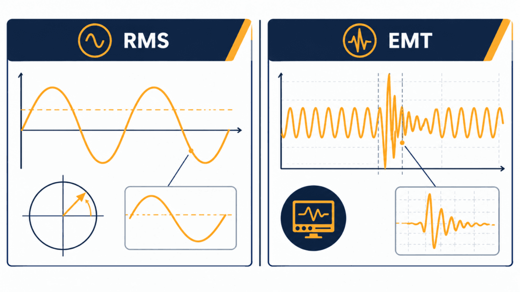
RMS and EMT are the two simulation domains used to study how a BESS plant behaves during a disturbance, not just at steady state. They answer different questions, at different levels of detail. A network operator usually specifies which one it needs based on how electrically weak the connection point already is.
First, RMS modelling stands for root-mean-square, or phasor-domain, simulation. It represents the network using simplified fundamental-frequency phasors. It tracks how power, voltage, and frequency evolve over seconds to minutes. So RMS is efficient enough to study a large interconnected network. It is the standard tool for frequency response, voltage stability, and wide-area planning work.
Conversely, EMT modelling stands for electromagnetic transient simulation. It represents the actual instantaneous waveform, not a simplified phasor. It captures behaviour on the scale of microseconds to milliseconds. Even so, EMT is far more demanding to compute, which limits it to a smaller network area. It is generally the preferred domain for capturing fast inverter control-loop interactions, detailed unbalanced-fault behaviour, switching transients, and other sub-cycle dynamics that a simplified RMS model may not capture adequately.
When EMT Modelling Becomes Necessary
A 2023 NERC reliability guideline on BESS and hybrid plant modelling identifies low short-circuit strength, interaction risk among multiple inverter-based resources, and grid-forming control as important situations where detailed EMT assessment may be appropriate. The final requirement stays project- and network-operator-specific. Still, RMS models stay adequate for most standard planning and screening work. Even so, network operators increasingly ask for both. RMS handles the broad system-wide screening. EMT handles the specific, electrically sensitive area near the new plant.
For the country-specific grid-code obligations these studies are designed to demonstrate, see our BESS Grid Codes and Compliance guide.
RMS vs EMT at a Glance
Factor
RMS (Phasor-Domain)
EMT (Electromagnetic Transient)
Time scale
Seconds to minutes
Microseconds to milliseconds
Represents
Simplified fundamental-frequency phasor
Actual instantaneous waveform
Typical use
Frequency response, voltage stability, wide-area planning
Weak-grid behaviour, control interactions, protection response
Network size
Large, interconnected systems
Smaller, localized network area
Computational cost
Lower
Considerably higher
Model source
Vendor-supplied standardised dynamic model
Vendor-supplied detailed EMT model
System Strength and Weak-Grid Considerations
System strength describes how firmly the local network holds its voltage and frequency steady when a disturbance hits. A weak point of connection has relatively high impedance. That makes it more sensitive to fast inverter-control action, not less.
Indeed, a BESS can genuinely help a weak grid, especially with a well-designed voltage-control or grid-forming PCS. But connecting at a weak point still raises real risks. The study package needs to catch control-loop instability in grid-following inverters, conflicts between current limits and voltage support, harmonic amplification, and slower fault ride-through than a stronger point would show.
Grid-Forming Controls Don’t Automatically Fix a Weak Grid
Grid-forming capability has to be assessed against three things: the specific operating mode the network operator requires, the protection design, and how the plant interacts with other inverter-based resources nearby. It is one mitigation option among several, not an automatic pass. Our Australia BESS grid connection guide covers how one network operator assesses system strength and grid-forming capability in practice, including where AEMO’s own guidance applies.
How BESS Grid Connection Studies Fit Into the Interconnection Timeline
These study types do not run on their own. They sit inside one defined stage of the wider interconnection process. That stage generally follows the initial application and feasibility screening, but comes before a formal connection agreement. Our BESS interconnection process guide covers this full sequence step by step. The country guides for Australia, the UK, and Europe each show how local network operators schedule this stage in practice.
What a Developer Must Supply for BESS Grid Connection Studies
The network operator cannot run a meaningful study without accurate models from the project side. A model that does not match the as-built equipment is one of the most common reasons a study result later fails to match real commissioning-test behaviour. A typical model-deliverable package includes:
PCS RMS model in the network operator’s required format
EMT model, where requested or reasonably anticipated
Plant-controller model and parameter file
Inverter control-mode descriptions and operating limits
Transformer vector group, impedance, tap range, and grounding data
Cable and collector-system parameters
Protection single-line diagram and proposed relay settings
Reactive-power capability curve
Harmonic emission spectrum or equivalent frequency-domain data
Firmware, model, and controller version numbers
Model validation report and revision history
Common Pitfalls in BESS Grid Connection Studies
Most delays in a BESS grid-study package trace back to a small set of recurring issues. In fact, few come from a genuinely hard technical problem.
Common Study Failures and How to Avoid Them
Failure
Why It Happens
How to Prevent It
Studies start with only generic inverter data
The selected PCS or control configuration isn’t final yet
Use generic data for early screening only; replace it with validated project-specific models before final submission
Charging mode gets treated as secondary
Teams model export in detail but skim over maximum import and reactive-only cases
Include charging, discharging, standby, and reactive-only cases from the start
Co-located equipment gets left out
Nearby solar, capacitor banks, and cables all shift the dynamic and harmonic picture
Model the full plant and any electrically relevant equipment nearby
A model is submitted unvalidated
The network operator can’t reproduce the plant’s expected behaviour
Require validation evidence and parameter traceability from the PCS supplier
Late firmware changes go unreported
The installed controls no longer match the approved model
Use formal change control, and resubmit for study when material settings change
How Study Results Affect BESS Cost and Revenue
Grid connection studies aren’t just a technical hurdle; instead, their results feed straight into the project’s business case. A study can change several things at once. The substation and protection scope. The PCS rating actually needed. Whether harmonic filtering or extra reactive-power equipment gets added. The final export or import capacity the plant is allowed.
A project designed around a 100 MW PCS might come out of studies with only 80 MW of firm export capacity. Or it might carry a reactive-power reservation that reduces available active power at certain voltage conditions. Each of those changes affects CAPEX, usable revenue capacity, and lifetime project economics. So study results should inform the financial model before procurement is finalised, not after.
Do voltage and thermal limits hold with the plant connected?
Most grid-connected projects
Short-circuit
Fault condition
Does fault current stay within equipment and protection limits?
Common for projects requiring detailed technical review
Protection coordination
Fault response
Does protection stay selective and secure with the BESS added?
Where protection settings, fault duty, or anti-islanding could be affected
Harmonics
Waveform quality
Does distortion stay within planning levels at the connection point?
Common for inverter-based systems, where required by the operator or power-quality standard
RMS/EMT dynamic
Transient/dynamic
Does the plant stay stable through disturbances and control interactions?
More likely for large, weak-grid, grid-forming, or transmission-connected projects
Frequently Asked Questions
Common questions readers ask about BESS grid connection studies, answered directly.
Does every BESS project need all of these grid connection studies?
Not always. Smaller distribution-connected projects on a strong network often only need load flow, short-circuit, and protection coordination studies. Harmonics and dynamic RMS/EMT studies become more likely as project size grows, as the connection point gets weaker, or as the project uses grid-forming controls. Confirm the required scope with the relevant network operator.
Who actually performs BESS grid connection studies?
The network operator, or transmission owner, typically runs the studies. It uses models the developer’s equipment vendors and system integrator supply. Some markets let a developer commission an independent, accredited study provider for part of the work, subject to the operator’s review.
What’s the real difference between RMS and EMT modelling?
RMS modelling represents slower power-system dynamics using simplified phasors. In contrast, EMT modelling represents the actual instantaneous waveform, capturing much faster behaviour down to microseconds. EMT suits weak-grid and control-interaction studies that RMS cannot see in enough detail.
Why does a BESS need its own short-circuit study, instead of using generic generator data?
A battery inverter’s fault current is limited by its control system, not by machine impedance, so it behaves differently from a synchronous generator during a fault. Reusing generic synchronous-generator assumptions for a BESS can misrepresent both the maximum and minimum fault-current cases that protection settings depend on.
How long does a full grid connection study package take?
Timelines vary by market, network operator workload, and study complexity. They can range from a few weeks for a simple load flow and short-circuit package, to many months where full RMS and EMT modelling is required. Treat any timeline as a planning estimate, and confirm current queue times with the relevant network operator.
What happens if a project fails a grid connection study?
A failed result rarely ends the project outright. So the network operator usually proposes a fix instead, such as a lower export limit, added reactive power support, network reinforcement, or a different control-mode requirement. The project is then re-studied against the revised assumptions. Rejection outright is uncommon in real BESS grid connection studies.
Do harmonics studies apply differently to a BESS than to solar PV?
The underlying inverter switching behaviour is similar. But a BESS charges and discharges across a four-quadrant range, so its harmonic contribution needs checking across a wider set of operating points than a generation-only solar PV plant, which only ever exports.
Does a grid-forming BESS need a different study approach?
Often, yes. Grid-forming BESS projects are more likely to require detailed EMT assessment, because control-loop, current-limit, and fault-response behaviour can matter a great deal in weak-grid conditions. RMS modelling may still cover the broader system studies, but the network operator may separately require EMT evidence for the local interaction assessment.
Can a firmware update trigger a new grid connection study?
Yes. If a firmware change alters protection behaviour, current limits, grid-forming logic, fault ride-through, or reactive-power control, the network operator may require a fresh assessment or an updated model. Treat firmware updates on commissioned equipment as controlled engineering changes, not routine maintenance.
Glossary
More Sunlith Energy definitions for terms used throughout this BESS grid connection studies guide.
Study and Network Terms
Load flow (power flow) study — A steady-state check of voltage and equipment loading across the network, with a new plant connected.
Short-circuit (fault-level) study — A check of fault current magnitude at points across the network, used to confirm equipment and protection ratings.
POI (point of interconnection) — The physical point where a generating plant connects to the wider network.
PCC (point of common coupling) — The point on the network, often the same as the POI, where harmonic and power-quality limits get assessed.
System strength — How firmly a local network holds voltage and frequency steady when a disturbance occurs; a low-strength, or “weak,” connection point is more sensitive to fast inverter-control action.
Modelling and Power-Quality Terms
RMS modelling — Phasor-domain simulation used to study slower power-system dynamics, over seconds to minutes.
EMT modelling — Electromagnetic transient simulation used to study fast, instantaneous waveform behaviour.
THD (total harmonic distortion) — The RMS value of harmonic voltage (or current) components relative to the fundamental. Commonly used for voltage distortion at the connection point.
TDD (total demand distortion) — RMS harmonic current relative to the maximum demand load current, not the instantaneous fundamental current. IEEE 519 commonly uses this for current distortion.
Disclaimer
Important: This guide is general technical information, not project-specific engineering advice. Study requirements, thresholds, and timelines vary by network operator, connection voltage, project size, and jurisdiction. Confirm the required study scope and current standards with the relevant network operator, and a qualified electrical or grid-connection engineer, before relying on any figure here for a real project.
Further Reading
More Sunlith Energy guides on BESS interconnection, grid codes, and short-circuit standards.
A Europe BESS grid connection depends on the country where the project is located within the European Union, not just its size or voltage. The EU-wide Requirements for Generators (RfG) regulation provides a common technical baseline. But each country runs its own transmission system operator, its own national grid code, and its own connection process. So the practical route, and the risk of delay, can differ sharply between markets that share the same underlying EU rules.
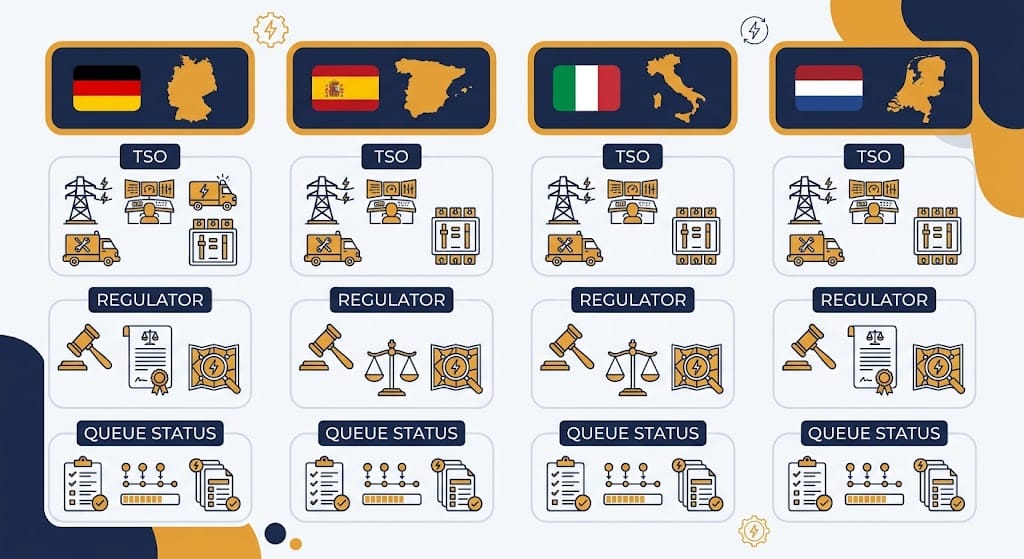
Scope note: This guide covers the EU-wide RfG framework, then spotlights four of Europe’s largest BESS markets: Germany, Spain, Italy, and the Netherlands. The United Kingdom sits outside the EU and follows its own framework, covered in a separate guide. Norway and Switzerland connect into the same ENTSO-E system but sit outside the EU too, and are not covered in detail here.
Quick answer: A BESS grid connection in the EU starts with the Requirements for Generators (RfG) framework, but the real route is decided nationally. The relevant TSO or DSO applies its own country-specific grid code, connection process, capacity-allocation rules, studies, and compliance tests. Germany, Spain, Italy, and the Netherlands each face significant connection pressure right now, so confirm current queue, congestion, and permitting requirements with the relevant network operator before fixing a schedule or equipment specification.
So, this guide walks through:
How the EU-wide RfG framework sets a common technical baseline across member states
Who governs a Europe BESS grid connection at the EU level and the national level
How the connection process generally works, stage by stage
Country spotlights on Germany, Spain, Italy, and the Netherlands
The common thread across these markets, and how to reduce connection risk
Europe BESS Grid Connection Checklist
Confirm the country, connection voltage, network level, and applicable synchronous area, because RfG thresholds and national requirements vary.
Identify the likely RfG Power Generating Module Type (A, B, C, or D) for the project’s capacity and voltage.
Confirm whether the project connects to the national TSO or a regional DSO, and what that changes.
Check the national grid code’s specific requirements, since these can go well beyond the EU baseline.
Screen the country’s current connection-queue status, since several markets have overhauled their rules recently.
Ask the PCS supplier and system integrator for validated models in the format the network operator requires.
Allow schedule contingency for studies, national permitting, and grid-code compliance testing.
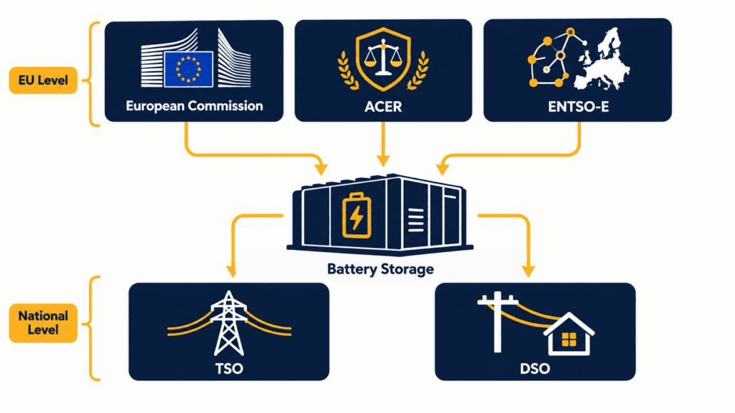
Who Governs a Europe BESS Grid Connection?
No single body runs a Europe BESS grid connection from end to end. Instead, EU-level bodies set the common framework, while national bodies run the actual connection process.
Organisation
Main role for BESS projects
European Commission
Adopts EU network codes, including RfG, as binding regulations across member states.
ACER
The EU Agency for the Cooperation of Energy Regulators. Recommends network codes and coordinates national regulators.
ENTSO-E
The European Network of Transmission System Operators. Coordinates technical implementation of RfG and related codes across national TSOs.
National TSO
Operates the transmission grid and connects larger or transmission-voltage projects. The number and structure of TSOs vary by country; Germany, for example, has four.
National DSO(s)
Operate regional or local distribution networks and connect most smaller and medium-sized projects. Often several per country.
National regulator
Approves connection rules and technical codes at the national level. Examples include Germany’s Bundesnetzagentur, Spain’s CNMC, Italy’s ARERA, and the Netherlands’ ACM.
So don’t assume ENTSO-E or the European Commission reviews individual projects. Instead, they set the common framework. In practice, the project deals mainly with the relevant TSO or DSO and, where applicable, the energy regulator.
The EU-Wide Framework Behind a Europe BESS Grid Connection
RfG classifies Power-Generating Modules (PGMs) into Types A to D. For BESS projects in EU member states, this is the shared technical baseline behind most connection requirements.
Type
General basis
What it means in practice
Type A
Smallest capacity, lowest voltage
Fewest technical requirements, often a simplified process
Type B
Small to medium capacity
More technical requirements than Type A, thresholds vary by country
Type C
Medium to large capacity
Detailed technical and testing requirements
Type D
Largest capacity, or connects at high voltage
Most extensive requirements, including full system studies
The exact MW thresholds between types are not identical across the EU, though. RfG sets upper limits for each synchronous area, but leaves the precise threshold within that band to the national level. So a project sitting near a threshold in one country may fall into a different type in another. Confirm the applicable type with the connecting TSO or DSO rather than assuming a single EU-wide number.
Battery storage adds a further wrinkle, and this is worth reading carefully. RfG was drafted around generation, and storage can be treated differently depending on the national implementation, the BESS’s operating mode, and its connection arrangement. In many member states, storage that exports to the grid is assessed using requirements aligned with the relevant PGM category, but developers should confirm the exact national treatment with the connecting TSO or DSO rather than assume it works identically to a conventional generator. National implementation of RfG can also add significant detail beyond the EU baseline, as our global BESS grid codes comparison shows.
How the Europe BESS Grid Connection Process Works, Stage by Stage
Treat the connection journey as a set of stages, not one checklist. The framework stays similar across countries, but the pace and detail vary a great deal, as the country spotlights below show.
Stage 1: Site Screening and Capacity Assessment
First, confirm the country, the likely point of connection, and whether that point sits on the transmission or distribution network. Then estimate the project’s likely RfG type, since this shapes both the technical requirements and the study scope ahead. Also screen the national connection queue early. As the country spotlights below show, several major markets are running queues many times larger than their planning assumptions. So realistic timing matters more than nameplate capacity alone.
Stage 2: Connection Application
Next, submit a connection application to the relevant network operator. That means the relevant TSO for transmission-network connections or larger projects, or the relevant DSO for many distribution-network connections. The application should identify the proposed site, capacity, connection voltage, and intended operating modes. Requirements for what to include vary by country, so check the specific network operator’s current application format rather than assuming one EU-wide template.
Stage 3: Studies and Compliance Verification
The network operator then sets the study scope. Larger or higher-type projects generally need load-flow, short-circuit, and dynamic-performance studies against the applicable national grid code. Many countries also require compliance documentation, certificates, or witnessed test evidence before energisation, where the national framework calls for it, confirming the installed plant meets the agreed technical requirements.
Treat model submission as real engineering, not paperwork. Ask the PCS supplier and system integrator for validated models in the format the network operator requires, together with controller logic and operating-mode assumptions, before finalising procurement.
Both the network operator’s response and the surrounding permitting process vary significantly by country. In some markets, access and connection authorisations are processed through linked or coordinated procedures. In others, they are separate stages with their own timelines. Environmental and planning permits often run in parallel, and can end up the longer critical path on a large project. Confirm the current sequence with the relevant network operator and permitting authority early.
Stage 5: Construction and Commissioning
Commissioning confirms the installed plant matches the approved design. Expect to provide as-built documentation and protection settings, plus any certification or compliance evidence required by the national framework and network operator before energisation. Testing typically covers protection behaviour and, for larger or higher-type projects, dynamic performance against the applicable grid code.
Stage 6: Ongoing Compliance
Compliance does not stop once operation begins. Instead, changes to inverter firmware, protection settings, plant-controller logic, or other declared technical parameters can trigger a reassessment. So treat compliance documentation as an ongoing operational task, not a one-off commissioning step.
Realistic timelines vary enormously by country and by where a project sits in that country’s connection queue, application pipeline, or capacity-allocation process. A small, distribution-connected project can sometimes progress in months. A large, transmission-connected project in a congested market can take years, and several major markets are actively reworking their queue rules as this guide is written. Build schedule contingency around studies and queue position specifically, since both are the hardest parts to forecast right now.
Germany runs four regional TSOs: 50Hertz, Amprion, TenneT Germany, and TransnetBW. Their number and structure are specific to Germany, not a Europe-wide pattern. Distribution-level projects instead connect through one of many regional DSOs. The national regulator is the Bundesnetzagentur.
Technical requirements come from the VDE-AR-N series: 4105 for low voltage, 4110 for medium voltage, and 4120 for high voltage, each implementing RfG in German-specific detail. Battery projects also typically need to meet VDE-AR-E 2510-50 for battery safety, alongside the relevant grid-connection code.
The connection process itself is changing. By the end of Q3 2025, Germany’s four TSOs had received 545 applications for large battery-storage systems representing 211 GW of requested capacity. That figure describes application volume, not contracted or construction-ready capacity, and it compares to a Grid Development Plan forecast of just 41 to 94 GW of large-scale storage by 2037.
In response, the TSOs jointly proposed a new maturity assessment procedure, the Reifegradverfahren, to move away from allocation based solely on application date, toward an evaluation based on land control, permitting status, technical readiness, and financial or commercial readiness. The procedure began its application phase on 1 April 2026. As of that announcement, the TSOs themselves noted that confirmation of the procedure’s legal basis by the Bundesnetzagentur was still advisable. So treat this as a live, TSO-led process still being formalised, rather than a settled legal framework, and confirm current requirements directly with the relevant TSO.
Spain has one national TSO, Red Eléctrica de España (REE), plus regional DSOs for distribution-level connections. Meanwhile, the national regulator is the Comisión Nacional de los Mercados y la Competencia (CNMC).
Since 2020, Spain has processed access and connection permits together. Developers submit a single joint application to REE or the relevant DSO, rather than two separate steps. During 2025, Spain’s storage-access framework underwent several changes. Royal Decree-Law 7/2025 included proposed measures relevant to storage access, but Congress rejected it on 22 July 2025, so it never took permanent legal effect. Related provisions were later introduced through Royal Decree 997/2025, approved on 5 November 2025, which also addressed how installed capacity is calculated for hybrid and standalone storage projects. Given this history, confirm the currently applicable rule directly with REE or CNMC rather than citing either decree from memory.
The scale of pent-up demand is striking. Published Spanish grid data has indicated a large pipeline of storage projects at different access, connection, and pre-commissioning stages, while commissioned battery capacity remains much lower, on the order of a few hundred MW. Check REE’s latest dataset before using any specific pipeline figure in a schedule or investment decision.
In Italy, Terna manages transmission-network connections, while regional distribution operators manage most distribution-network connections. In some circumstances, projects of 10 MW or more may be handled by Terna, but the responsible operator depends on the point of connection, voltage level, network configuration, and the applicable TICA provisions. ARERA, the national energy regulator, sets the technical and economic conditions for both, through the Testo Integrato delle Connessioni Attive (TICA). Confirm the route with the prospective network operator rather than relying on capacity alone.
Like Germany and the Netherlands, Italy is managing far more connection requests than its network was planned for. As of 31 May 2026, Terna’s Econnextion platform recorded roughly 294 GW of storage connection requests alone, well beyond national 2030 targets. In response, Decreto MASE 291/2026, signed 8 September 2026 and in force from 9 September 2026, requires Terna to divide the national transmission grid into microzone (microzones) and calculate available capacity for renewables and storage within each. The decree sets out a phased rollout: Terna must submit its microzone methodology to the ministry within 30 days of the decree taking effect, with the finalised microzones published within a further 15 days after approval. So treat the underlying capacity-allocation reform as legally in force, but the actual microzone boundaries and published capacity figures as still being rolled out through late 2026.
The Netherlands has one national TSO, TenneT, plus regional DSOs for distribution-level connections. The Authority for Consumers and Markets (ACM) is the national regulator.
Grid congestion, known locally as netcongestie, is the defining issue for new connections in much of the country. TenneT’s own reporting has described a connection queue including tens of gigawatts of battery storage requests against a national peak load a fraction of that size.
In response, ACM authorised flexible capacity arrangements, including what TenneT calls the time-bound transmission right (TDTR) and the capacity control contract (CSC), under which a project may accept reduced or conditional access in exchange for network capacity or congestion-management value. A battery that can act as a controllable congestion mitigator, reducing strain on the grid at TenneT’s request under this framework, may receive preferential treatment under the applicable congestion-management or capacity-allocation framework. Confirm the exact contract type, availability, and eligibility conditions directly with TenneT or the relevant DSO, since this framework is still being extended to new regions and projects.
Comparing Europe BESS Grid Connection Markets: Germany, Spain, Italy, and the Netherlands
Country
Transmission operator
Main connection issue
Check first
Germany
4 regional TSOs
High application volume, new maturity-based allocation
Applicable TSO’s current process and connection point
Spain
REE
Unsettled storage-access rules, large pending pipeline
REE/DSO access capacity and current permit route
Italy
Terna + regional DSOs
Capacity allocation via new microzone system
Connection voltage and responsible operator
Netherlands
TenneT + regional DSOs
Widespread congestion (netcongestie)
Firm versus flexible capacity options
The Common Thread Across These Europe BESS Grid Connection Markets
Germany, Spain, Italy, and the Netherlands look different on the surface. Each has its own TSO structure, its own national code, and its own institutions. But they share a pattern worth noticing. Across all four, high volumes of storage and hybrid-project applications have increased pressure on connection processes. Network operators are increasingly using readiness evidence, technical feasibility, conditional-access arrangements, or other prioritisation tools, rather than relying solely on application date. The details differ materially by country and operator, and some of these changes are still being finalised as this guide is written.
For developers, that means two things. First, don’t plan a European BESS project around queue rules you read about even a year ago; they may already be out of date. Second, a project’s evidence of real readiness, land control, permits, financing, and validated technical models, increasingly matters as much as when it first applied.
Common Risks in a Europe BESS Grid Connection
Most delays in a Europe BESS grid connection trace back to a small set of repeat mistakes. So here is how to catch them early.
Risk
Consequence
Mitigation
Assuming one EU-wide threshold or process applies
Wrong compliance pathway assumed early
Confirm the national RfG type and process with the specific TSO or DSO
Relying on outdated queue-rule guidance
Schedule built on a process that no longer applies
Check current queue and prioritisation rules directly with the network operator
Selecting a site before checking congestion status
Non-firm terms or multi-year delay
Screen the country’s current congestion and queue data early
Incomplete or unvalidated dynamic models
Delayed studies and commissioning rework
Require validated models from the PCS vendor and integrator
Treating national code compliance as an afterthought
Design changes late in development
Confirm the applicable national grid code early in concept design
Assuming permitting and connection run on the same timeline
Land, environmental, or planning delays block an otherwise-ready connection
Run permitting and connection work in parallel from the start
Planning a BESS project in Europe? Start with a country-specific connection-readiness assessment. Cover the applicable RfG type, national grid code, current queue status, and permitting timeline, before you finalise equipment specifications.
Frequently Asked Questions About a Europe BESS Grid Connection
Common questions developers ask before choosing a European market or signing a connection agreement.
Does one EU grid code cover every country?
No. RfG sets a common EU-wide baseline, classifying projects into Types A to D. But each country implements it through its own national grid code, which can add significant detail, as Germany’s VDE-AR-N series shows. Confirm the national code alongside RfG, not instead of it.
Is the UK covered by this Europe BESS grid connection guide?
No. The UK sits outside the EU and follows its own framework, built around NESO, the Grid Code, and Engineering Recommendations G98/G99/G100. See our dedicated UK guide for that detail.
Which European countries have the longest BESS connection queues right now?
Germany, Italy, Spain, and the Netherlands have all reported connection queues many times larger than their official capacity targets. Each has introduced new prioritisation rules within the past two years to manage this, so treat queue length as a moving target, not a fixed number.
Does battery storage get classified the same way as solar or wind under RfG?
Often, but not automatically. Many national frameworks apply Type A-D-style requirements to BESS when it exports to the grid, but the applicable classification can depend on the country, operating mode, hybrid configuration, and connection arrangement. Confirm the route with the connecting TSO or DSO.
Why do Germany, Italy, and the Netherlands all have such large storage queues?
Developers in each market applied for far more grid capacity than the underlying network was planned to carry. Partly, that happened because reserving a queue position cost little relative to a project’s potential value. All three countries have since introduced readiness or maturity-based rules to filter for projects genuinely likely to proceed.
Can a battery help resolve grid congestion instead of just adding to it?
In some markets, yes. The Netherlands’ congestion-mitigator framework, for example, lets a battery accept flexible or conditional access in exchange for helping manage congestion at the network operator’s request. Similar flexible-connection concepts are emerging elsewhere in Europe too.
How long does a Europe BESS grid connection take?
It varies enormously by country and by position in the relevant queue or pipeline. A small distribution-connected project can sometimes progress in months. A large, transmission-connected project in a congested market can take years, particularly in markets still working through a legacy backlog.
Do I need compliance certification before energising?
In many European countries, yes, particularly for larger or higher-type projects. Requirements vary by country and by RfG type, so the specific certification and testing route is best set early, with the connecting network operator.
Glossary of Terms for This Europe BESS Grid Connection Guide
Because this guide spans several countries, here are the key terms and institutions, defined in plain terms.
EU-Level Terms and Institutions
RfG — Requirements for Generators — Regulation (EU) 2016/631, the EU network code establishing baseline requirements for connecting Power-Generating Modules. National frameworks may apply related requirements to battery storage depending on the project’s operating mode and connection arrangement.
ENTSO-E — European Network of Transmission System Operators for Electricity — coordinates technical implementation of RfG and related codes across national TSOs.
ACER — EU Agency for the Cooperation of Energy Regulators — recommends network codes and coordinates national energy regulators.
PGM — Power-Generating Module — a generating unit or group of generating units covered by the applicable connection requirements. Under RfG, PGMs are assigned Type A, B, C, or D requirements according to the applicable capacity, voltage, and national criteria.
Synchronous area — A group of interconnected power systems operating in synchronism at the same nominal frequency. RfG thresholds may differ by synchronous area.
National Institutions Referenced in This Guide
TSO — Transmission System Operator — the national (or, in Germany, regional) body that owns and operates the high-voltage transmission grid.
DSO — Distribution System Operator — the regional or local body that owns and operates the lower-voltage distribution network.
Bundesnetzagentur — Germany’s national energy regulator, which oversees grid connection rules and the country’s four TSOs.
CNMC — Spain’s national markets and competition regulator, which approves technical criteria for grid access alongside REE.
ARERA — Italy’s national regulator for energy, networks, and the environment, which sets connection rules through the TICA.
ACM — The Netherlands’ Authority for Consumers and Markets, which regulates grid congestion and connection-priority rules.
Important: This guide is general information, so treat it that way, not as legal, engineering, or connection advice. Grid-compliance requirements vary by country, network operator, project design, and the applicable rules at the time of assessment. Several of the markets covered here are actively reforming their connection processes. Confirm requirements with the relevant national TSO or DSO, national regulator, and qualified electrical, grid-connection, and legal advisers.
Further Reading on Europe BESS Grid Connection
More Sunlith Energy guides on battery storage connection, interconnection, and compliance.
A UK BESS grid connection depends on the connection voltage, export capacity, site location, network operator, and the project’s status in the connections queue. Smaller distribution-connected systems commonly follow a DNO-led Engineering Recommendation G98 or G99 process. Larger embedded and transmission-connected projects, by contrast, may need more extensive system studies, Grid Code compliance, CUSC arrangements, and a place in the reformed connections process. So a battery is never approved just because its inverter rating matches the site.
Scope note: This guide covers BESS projects connecting in Great Britain (England, Scotland, and Wales), regulated by Ofgem and coordinated by NESO. Northern Ireland operates under a separate regulatory system, as part of the Single Electricity Market with Ireland, which this guide does not cover in detail.
Quick answer:
A UK BESS grid connection depends on connection voltage, export capacity, location, and where the project sits in the connections queue. Smaller, distribution-connected batteries typically go through an Engineering Recommendation G98 or G99 application with the local DNO. Larger or transmission-connected projects usually need a Bilateral Connection Agreement, Grid Code compliance, and a place in NESO’s reformed connections pipeline.
So, this guide walks through:
How NESO, Ofgem, DNOs and Transmission Owners each fit into a BESS interconnection
The difference between distribution-connected (G98/G99/G100) and transmission-connected pathways
The stage-by-stage connection process, including NESO’s 2025 Connections Reform
Grid Code requirements for Electricity Storage Modules
UK-specific technical challenges and common project risks
UK BESS Connection Checklist
Identify the likely point of connection and confirm distribution versus transmission voltage.
Check whether the proposed installation falls within the applicable G98 current limit and notification conditions.
Confirm the project’s status and expected offer window under NESO’s Connections Reform pipeline.
Screen local network constraint and curtailment risk for the specific region.
Confirm the applicable Grid Code Power Generating Module Type and its technical requirements.
Ask the PCS supplier and system integrator for the model format the network operator requires, such as RMS or EMT, together with validated parameters, controller logic, and operating-mode assumptions, before finalising procurement.
Allow schedule contingency for studies, Bilateral Connection Agreement negotiation, and commissioning.
Who Governs a UK BESS Grid Connection?
No single body runs UK BESS approval from start to finish. Instead, several organisations share the job, and the reformed connections process has changed how a few of them work together.
Organisation
Main role for BESS projects
NESO
Great Britain’s electricity system operator. Coordinates the reformed transmission-connection process and works with Transmission Owners and DNOs on queue reform and connection offers. For many distribution-connected projects, the relevant DNO remains the main counterparty, not NESO directly.
Ofgem
Independent regulator for Great Britain. Approves code changes such as the Connections Reform modifications and regulates network company price controls.
Transmission Owners
Build and maintain the transmission network. Examples include National Grid Electricity Transmission (England and Wales), SP Transmission and Scottish Hydro Electric Transmission (Scotland).
DNOs and iDNOs
Assess and connect distribution-level projects. They process G98 and G99 applications, set local protection and export-limit conditions, and increasingly act as Distribution System Operators managing local network capacity.
So don’t assume NESO reviews every battery project directly, and don’t assume it runs a single unified pipeline on its own. Smaller, distribution-connected batteries mostly deal with their DNO, so keep that relationship central throughout.
Distribution vs. Transmission: Two Paths for a UK BESS Grid Connection
One factor shapes grid approval more than any other: where the asset physically connects, and at what voltage. Distribution and transmission pathways lead to very different applications and timelines.
Factor
Distribution-connected BESS
Transmission-connected BESS
Typical use case
C&I storage, community batteries, smaller grid-scale projects
Utility-scale storage, large co-located projects
Main counterparty
DNO or iDNO
NESO and the relevant Transmission Owner
Governing framework
EREC G98, G99, and G100
Grid Code, CUSC, and a Bilateral Connection Agreement
Technical focus
Export limits, protection, voltage rise, anti-islanding
Power Generating Module Type, dynamic performance, system studies
Key risk
Local network constraint, DNO queue position
Connections Reform pipeline position, study timelines
Project size alone doesn’t decide the pathway, though. A regional quirk matters here. In parts of Scotland, an embedded project as small as 30 MW can need a Bilateral Connection Agreement and CUSC party status. A similarly sized project in England or Wales, by contrast, may fall under the Licence Exempt Embedded Medium Power Stations arrangement instead. So confirm the specific threshold with the relevant network operator, rather than assuming a single GB-wide MW cut-off. More broadly, the categories in the table above are general planning distinctions, not universal legal classifications. A distribution-connected project can still carry Grid Code, CUSC, or transmission-system obligations depending on its configuration. So confirm the applicable route with the DNO, NESO, and the relevant Transmission Owner.
The UK BESS Grid Connection Process, Stage by Stage
Treat the connection journey as a set of stages, not one checklist. Each stage builds on the last, and the 2025 Connections Reform changed how several of them work.
Stage 1: Site Screening and Capacity Assessment
First, check the site’s real limits before you lock in battery duration or PCS (power conversion system) rating. Review available capacity at the likely connection point. Then confirm whether the project falls within the applicable G98 current limit and notification conditions, or whether it will need a full G99 application instead. Next, assess local network constraint, since some regions are heavily congested for new BESS capacity, and a few areas have effectively closed for certain technologies.
Also map planning consent requirements and any land or grid-easement issues early. A connections queue position can take months to secure, so running planning and land work in parallel avoids a stacked delay later in the schedule.
Stage 2: Connection Application
Next, submit the applicable connection application. For distribution-connected projects, this usually means an EREC G99 application to the local DNO, identifying the proposed site, export capacity, inverter specifications, and intended operating modes. For larger or transmission-connected projects, this instead means an application to NESO. That application now sits inside the reformed Connections Reform pipeline, rather than the old first-come, first-served queue.
Stage 3: Studies and Queue Position
The network operator then sets the study scope for the project. Distribution-connected projects may need protection-coordination, voltage-rise, and export-limit studies. Larger or transmission-connected projects may also require load-flow, short-circuit, and dynamic-performance studies against the applicable Grid Code requirements.
Since 10 June 2025, eligible transmission-connected and some larger embedded projects are also assessed under NESO’s reformed connections framework, commonly known as TMO4+ (Target Model Option 4 Plus). Under this framework, a project earns a Gate 2 connection date and queue position by meeting defined readiness criteria and passing a strategic-alignment check. That replaces the old rule of holding a position by application date alone. Projects with existing agreements go through a one-off reassessment called Gate 2 to Whole Queue (G2TWQ). For small and medium embedded generators, NESO issues a Gate 1 offer to the DNO first, and the DNO takes it from there. The precise process depends on the project’s connection route, capacity, application status, and the relevant network operator. So confirm current requirements directly with NESO or the DNO, rather than assuming every project follows an identical path.
Stage 4: Connection Offer and Agreement
For distribution-connected projects, this stage produces the DNO’s response to a G98 or G99 application. Depending on the project and DNO process, that response may take the form of an acceptance, technical offer, connection offer, or approval subject to specific documentation. Either way, it sets out technical conditions and any required network reinforcement. For transmission-connected or larger embedded projects, this stage instead produces a Bilateral Connection Agreement. That agreement binds the project to the Connection and Use of System Code (CUSC) and the applicable Grid Code requirements. Offer timing now depends on the project’s phase and queue position under Connections Reform. So confirm current expectations directly with NESO or the relevant DNO, rather than relying on older published timelines.
Stage 5: Design, Construction and Commissioning
Commissioning confirms the installed plant matches the approved design. So, first, expect to provide as-built drawings and protection settings. Then witness testing and G99 or Grid Code compliance testing follow, covering protection, anti-islanding, and, where applicable, dynamic-performance verification. Commissioning evidence and updated models may also be required before the DNO or NESO issues final approval to energise.
Stage 6: Ongoing Compliance
Compliance does not stop once operation begins. Instead, changes to inverter firmware, protection settings, control-system configuration, or export limits may trigger a reassessment. So, treat compliance documentation as an ongoing operational task, not a one-off commissioning step, since it protects the connection agreement over the plant’s full operating life.
Realistic timelines vary widely by project size and location. A straightforward G98 or small G99 connection may progress in a matter of months. But a transmission-connected or large embedded project now depends heavily on its position in the reformed connections pipeline. NESO’s own December 2025 results show the queue moving in phases through 2026 and beyond. Build schedule contingency around queue position and study timelines, since both remain genuinely difficult to forecast precisely during this transition period.
Grid Code Requirements for a UK BESS Grid Connection
Grid Code requirements sit at the technical centre of any transmission-connected or large distribution-connected UK BESS grid connection. The Grid Code and associated connection-code provisions include requirements specifically relevant to Electricity Storage Modules. These interact with the applicable Power Generating Module classification, connection voltage, capacity, and operating mode.
First, the Grid Code sorts Power Generating Modules, including storage, into Types A to D. The thresholds are the same across Great Britain, and they set the technical requirements each module must meet. Then, depending on the module type and connection arrangement, a project may need to become a CUSC party. Or it may instead qualify for a licence-exempt arrangement handled mainly through the Distribution Code. Which pathway applies depends on connection voltage, project size, and sometimes regional variation. So confirm the applicable module type and compliance route directly with NESO or the relevant network operator early in development.
Performance area
Why it matters for battery storage
Active-power control
The BESS must charge, discharge, and respond to dispatch instructions accurately.
Reactive-power capability
The plant may need to inject or absorb reactive power to support voltage.
Frequency response
Storage can respond fast, but the response must still match the relevant Grid Code obligations.
Fault ride-through
The plant may need to stay connected through defined voltage disturbances.
Protection
Settings must clear internal faults while avoiding unnecessary tripping for external events.
Dynamic performance
Validated models help confirm the plant behaves as designed under real system conditions.
Does Every BESS Need a Bilateral Connection Agreement?
No, not every project does. Whether a BESS needs a Bilateral Connection Agreement and CUSC party status instead depends on its connection voltage, capacity, and sometimes its specific region. The England/Wales-versus-Scotland threshold difference shows why. Smaller distribution-connected projects instead work through the relevant DNO under G98 or G99. Developers should confirm the applicable pathway during early site screening rather than rely on a single capacity threshold as a proxy.
G98, G99, and G100 for Distribution-Connected Batteries
For distribution-connected battery systems, Engineering Recommendations G98 and G99 are the core technical references, with G100 applying separately wherever export limitation is used. G98 covers connect-and-notify installations that meet specific current and equipment conditions, generally up to 16A per phase, roughly 3.68kW on a single-phase supply. Installations outside those conditions generally need a full G99 application, but the DNO should confirm the correct route for the proposed configuration rather than relying on capacity alone.
G100 applies where an export limitation scheme is used to restrict the power a site sends back to the distribution network. It is not specific to DC-coupled battery storage. A DC-coupled BESS may need to meet G98 or G99 requirements too, depending on the generating-unit and inverter configuration. And an export-limited connection normally needs a validated control scheme, metering arrangement, and fail-safe behaviour. The DNO needs to be able to rely on that behaviour if control, communications, or measurement fails. None of these Engineering Recommendations replace the DNO’s own connection agreement or local network conditions. Larger C&I or grid-scale battery projects should confirm export limits, protection requirements, and network reinforcement needs directly with the DNO. See our full BESS grid codes comparison for the country-by-country comparison, including how UK grid codes fit alongside other major markets.
A quick self-check before diving into the detail below.
Question
Likely implication
Is the system within the G98 current limit and notification conditions?
G98 connect-and-notify may apply
Is the system above those G98 limits or conditions?
A G99 assessment is likely
Does the project use an export limitation scheme?
G100-related requirements may apply, alongside G98 or G99
Is the project transmission-connected or a large embedded project?
NESO, the Transmission Owner, CUSC, Grid Code, and BCA requirements may arise
Is the project in the reformed connections queue?
Gate 1 or Gate 2 status and readiness evidence may affect timing
Technical Challenges Unique to a UK BESS Grid Connection
A few UK-specific conditions make grid approval harder here than a generic global playbook suggests. These conditions shape both design choices and realistic project timelines.
Connections Reform and Queue Position
As Stage 3 covers, readiness now matters as much as application date. NESO’s own reporting shows the pre-reform queue exceeded 700 GW, while the reformed pipeline instead prioritises a smaller, more deliverable set of projects. In practice, that means a project’s land rights, planning progress, and evidence pack can matter more to its timing than how early it applied.
Grid-forming capability: NESO has published dedicated technical guidance for grid-forming plant, including Electricity Storage Modules. In some locations, connection studies may consider whether grid-forming controls can support network stability. Grid-forming capability is not a substitute for a connection assessment, however. Its value depends on the network need, the plant’s control design, and the operating characteristics the project accepts. So treat it as one design input among several, not a fix on its own.
Network capacity for new BESS varies sharply by region. Some parts of Great Britain, including areas of Scotland, face significant constraint for new storage and generation capacity. So, in practice, a site’s regional location can matter as much as its technical design for realistic connection timing.
Curtailment and Commercial Risk
A connection offer may include a formal non-firm connection, active network management, or another constraint mechanism in congested areas. These are not all the same thing. Distribution export limitations, transmission constraint costs, and scheduled or dynamic curtailment can each apply differently depending on the connection. Because of this, test your revenue model against the specific curtailment terms in your own connection offer, not a generic assumption. Do this before you finalise the business case. A conservative revenue case, built around the connection offer’s real terms, protects the project from an optimistic forecast that never eventuates.
Common Risks in a UK BESS Grid Connection
Most delays in a UK BESS grid connection trace back to a small set of repeat mistakes. So here is how to catch them early.
Risk
Consequence
Mitigation
Assuming a single GB-wide MW threshold applies
Wrong compliance pathway assumed early
Confirm the applicable threshold with the specific network operator
Treating queue position as fixed by application date
Schedule built on outdated queue assumptions
Track readiness and Gate 2 status directly through NESO
Selecting a site before checking regional constraint
Unexpected non-firm terms or long delays
Screen regional network capacity early in site selection
Incomplete or unvalidated dynamic models
Delayed studies and commissioning rework
Require validated models from the PCS vendor and integrator
Treating Grid Code compliance as an afterthought
Design changes late in development
Confirm the applicable Power Generating Module Type early
Uncontrolled post-commissioning changes
Non-compliance or reassessment obligations
Set up formal change-control for firmware and protection settings
Planning a BESS project in the UK? Start with a connection-readiness assessment. Cover site capacity, regional constraint, the applicable Grid Code or G98/G99 pathway, and Connections Reform queue status, before you finalise equipment specifications.
Frequently Asked Questions About a UK BESS Grid Connection
Common questions developers ask before signing a connection agreement, answered directly.
Do I need G98 or G99 for a battery storage system?
It depends on the maximum design current per phase and the connection arrangement, not just battery nameplate capacity. Systems that meet the G98 current limit and notification conditions, generally up to 16A per phase (roughly 3.68kW single-phase), can usually connect-and-notify. Systems outside those conditions generally need a full G99 application instead. The assessment timescale varies by DNO and project complexity, so treat any indicative period as a planning estimate, not a guaranteed service window.
What is NESO’s Connections Reform and how does it affect BESS projects?
Connections Reform, approved by Ofgem on 15 April 2025 and live from 10 June 2025, replaced the old first-come, first-served queue with the readiness-based TMO4+ model. Eligible projects earn a Gate 2 connection date by meeting readiness criteria and passing a strategic-alignment check, rather than by application date alone. Projects with existing agreements go through a one-off reassessment called Gate 2 to Whole Queue. The precise process still varies by connection route and network operator.
Does every large BESS project need a Bilateral Connection Agreement?
Not automatically. As the regional-threshold note above explains, it depends on connection voltage, capacity, and sometimes region. Confirm the applicable pathway with the relevant network operator during early screening, rather than assuming a fixed MW cut-off.
What is G100 and when does it apply?
G100 applies where an export limitation scheme is used to restrict how much power a site sends back to the distribution network. It is not specific to DC-coupled battery storage; a DC-coupled BESS may still need G98 or G99 separately, depending on its configuration. Confirm the applicable route with the DNO.
Does Northern Ireland follow the same rules as Great Britain?
No. Northern Ireland operates under a separate regulatory system, as part of the Single Electricity Market with Ireland, with its own versions of the equivalent engineering recommendations. This guide focuses on Great Britain.
How long does a UK BESS grid connection take?
It varies widely. A straightforward G98 or small G99 connection can take months. A transmission-connected or large embedded project now depends heavily on its position in the reformed connections pipeline, which is still moving through its phased rollout.
What is system constraint and how does it affect BESS projects?
Network constraint describes limited capacity at a given location to accept new generation or storage. In constrained areas, a connection offer may come with curtailment terms or a non-firm connection, which developers should factor into their revenue modelling.
Can a battery connect without full export capability in the UK?
Yes, in some cases. A non-export or export-limited design under G100 can simplify the connection pathway, especially for smaller distribution-connected projects. However, the project generally still needs DNO approval. It also needs a validated control scheme, metering arrangement, and fail-safe behaviour the DNO can rely on if control, communications, or measurement fails.
Glossary of Terms for This UK BESS Grid Connection Guide
Because this guide leans technical, here are the acronyms used throughout, defined in plain terms.
Organisations, Codes, and Agreements
BESS — Battery Energy Storage System — the battery, inverter, and control equipment that stores and dispatches electricity.
NESO — National Energy System Operator — Great Britain’s independent electricity system operator, responsible for coordinating the reformed transmission connections process.
Ofgem — The independent regulator for Great Britain’s gas and electricity markets, which approves code changes such as the Connections Reform modifications.
DNO — Distribution Network Operator — the regional company that owns and operates the local electricity distribution network.
iDNO — Independent Distribution Network Operator — a licensed operator of a distribution network not owned by the regional DNO, often serving a specific site or development.
TO — Transmission Owner — the company that builds and maintains the transmission network in its region, such as National Grid Electricity Transmission or SP Transmission.
CUSC — Connection and Use of System Code — the industry code governing transmission connection and use-of-system arrangements in Great Britain.
BCA — Bilateral Connection Agreement — the formal agreement binding a transmission-connected or large embedded project to CUSC and Grid Code requirements.
PGM — Power Generating Module — the Grid Code classification (Types A to D) based on connection voltage and capacity, which sets a project’s technical requirements.
ESM — Electricity Storage Module — the Grid Code and connection-code term for a battery storage installation, which interacts with the applicable PGM classification.
Connection Types and Process Terms
G98 — The Engineering Recommendation for connect-and-notify generation and storage installations that meet specific current and equipment conditions.
G99 — The Engineering Recommendation requiring DNO approval before connection, for installations that fall outside G98 conditions.
G100 — The Engineering Recommendation covering export and import limitation schemes, applicable wherever a project limits what it sends to or draws from the network.
TMO4+ — Target Model Option 4 Plus — the readiness-based connections queue model introduced under the 2025 Connections Reform.
Gate 1 — An indicative connection offer stage, typically issued to the DNO for small and medium embedded generators under the reformed process.
Gate 2 — The stage at which a project earns a confirmed connection date, point of connection, and queue position, after meeting readiness and strategic-alignment criteria.
Important: This guide is general information, so treat it that way, not as legal, engineering, or connection advice. Grid-compliance requirements vary by network operator, project design, location, and the applicable rules at the time of assessment. The UK’s connections framework is also under active reform. Confirm requirements with the relevant DNO, NESO, Ofgem where applicable, and qualified electrical, grid-connection, and legal advisers.
Further Reading on UK BESS Grid Connection
More Sunlith Energy guides on battery storage connection, interconnection, and compliance.
Every Australia BESS grid connection follows its own path. There is no single national checklist. Requirements vary by jurisdiction, network provider, connection voltage, and project size. They also depend on system strength and whether the asset trades in the National Electricity Market. So a battery is never approved just because its inverter rating matches the site. Developers must also show the whole plant stays stable under normal and disturbed grid conditions.
Scope note: This guide focuses primarily on BESS projects connecting in the National Electricity Market (NEM), covering Queensland, New South Wales, the ACT, Victoria, South Australia and Tasmania. Western Australia and the Northern Territory operate separate electricity-market and network-connection arrangements, which this guide does not cover in detail.
Quick answer:
An Australia BESS grid connection depends on several things: connection voltage, export and import capacity, location, market participation, and the rules of the relevant network. Large, NEM-connected projects usually undergo detailed connection studies and project-specific performance-standard assessment. Smaller systems typically work with their DNSP, but may still need export controls, protection upgrades, or network-specific approval.
This guide walks through:
How AEMO, AEMC, AER, TNSPs and DNSPs each fit into a BESS interconnection
The difference between transmission- and distribution-connected pathways
The stage-by-stage connection process, including Generator Performance Standards
Australia-specific technical challenges, including system strength and control interactions
Common project risks and how to reduce them
Australia BESS Connection Checklist
Identify the likely point of connection and available import/export capacity.
Confirm whether the project is transmission-connected, distribution-connected, embedded, or behind the meter.
Screen local fault level, system strength, congestion, and curtailment risk.
Confirm the relevant registration, performance-standard, and connection-agreement pathway.
Obtain required OEM and integrator RMS and EMT model commitments before procurement.
Define the interface between the PCS, PPC, EMS, protection scheme, SCADA, and DNSP/TNSP controls.
Allow schedule contingency for study iterations, technical negotiations, remediation works, and commissioning evidence.
Who Governs an Australia BESS Grid Connection?
No single regulator runs the approval process start to finish. Instead, several bodies share the job. Each one controls a different part of the connection.
Organisation
Main role for BESS projects
AEMO
Operates the NEM and administers registration and connection-related processes under the National Electricity Rules. Its role in a given project depends on the asset’s registration status, connection pathway, and applicable performance-standard requirements.
AEMC
Writes the National Electricity Rules. These govern connection and market arrangements.
AER
Regulates network businesses and market conduct.
TNSPs
Assess connection applications, define required studies and technical conditions, and execute the connection agreement for transmission-scale projects. Examples include Transgrid, Powerlink, ElectraNet, AusNet and TasNetworks.
DNSPs
Assess connection applications, define required studies and technical conditions, and execute the connection agreement for distribution-connected projects. They also set local protection, metering and export-limit rules.
WA and NT bodies
Operate under separate market and regulatory structures, outside the NEM.
Don’t assume AEMO approves every battery. Instead, its role depends on the connection pathway and the project’s registration status. Either way, the connecting network business stays central to approval, so keep that relationship close throughout.
Current detail on each body’s role: AEMO, AEMC, AER.
Transmission vs. Distribution: Two Paths for an Australia BESS Grid Connection
One factor shapes grid approval more than any other: where the asset physically connects. Transmission and distribution pathways lead to very different studies and timelines. So, picking the right connection point early saves real time later.
C&I storage, community batteries, smaller utility projects
Main counterparty
TNSP
DNSP
Market relevance
Usually significant for registered NEM participants
May be exempt, embedded, or export-limited
Technical focus
Performance standards, system strength, network-wide models
Export capacity, protection, voltage rise, local feeders
Key risk
Long study cycles, changing negotiations
Limited export capacity, local upgrade costs
A behind-the-meter battery is not automatically simple, though. For example, if it can export, island, or materially alter site demand or network flows, the DNSP may still get involved. It can ask for studies, protection changes, or new operating limits.
The Australia BESS Grid Connection Process, Stage by Stage
Treat the connection journey as a set of stages, not one checklist. Each stage builds on the last. Skipping ahead usually costs time later.
Stage 1: Site Screening and Capacity Assessment
First, check the site’s real limits before you lock in battery duration or PCS (power conversion system) rating. Review available import and export capacity. Then confirm the connection voltage and the likely point of connection. Next, assess local fault levels, system strength, and nearby renewable congestion. Also check curtailment risk early, since it directly affects revenue.
Finally, decide whether the project will run non-exporting, export-limited, or under a dynamic operating envelope. Dynamic operating envelopes are an emerging and increasingly used option on parts of Australian distribution networks. Instead of a fixed export limit, some networks now offer a time-varying limit based on real conditions. Availability, control interfaces, and commercial implications vary by DNSP and connection type, so confirm what your specific network actually offers.
Also map the site’s land tenure, easements, and any planning-approval overlap early. A grid study can take months, so running it in parallel with land and environmental approvals avoids a stacked delay later in the schedule.
Next, submit a connection enquiry to the relevant network provider. The enquiry should identify the proposed site, point of connection, MW/MWh rating, intended operating modes, and requested import and export limits. Include the preliminary single-line diagram, inverter and transformer specifications, and any planned participation in energy, FCAS, demand-response, or backup-power functions.
Stage 3: Connection Studies
The network provider then sets the study scope for the project. Larger or more complex assets may require load-flow, short-circuit, harmonic, protection-coordination, and reactive-power studies. Where the connection is electrically weak, or where inverter interactions are material, the assessment may also require dynamic RMS (electromechanical, phasor-domain simulation) and EMT (electromagnetic-transient simulation) modelling.
Treat model submission as real engineering, not paperwork. The network assessment may depend on models for the PCS, plant power controller, EMS interfaces, transformers, protection systems, and the integrated BESS plant, not the PCS alone. Require the relevant OEMs and system integrator to supply validated RMS models and, where required, EMT models compatible with the relevant NSP or AEMO study environment, before finalising supply contracts.
For projects subject to the applicable NER performance-standard framework, this stage establishes the plant’s Generator Performance Standards. These obligations are developed through the connection process with the connecting TNSP or DNSP, with AEMO involved where the National Electricity Rules require it. GPS is not a generic battery standard: it reflects the applicable rules, the site’s network conditions, and the final BESS design. Negotiation can run for several months on a complex site, so start the GPS conversation well before financial close, not after it.
Stage 5: Design, Construction and Commissioning
Commissioning confirms the installed plant matches the approved design. So, first, expect to provide as-built drawings and protection settings. Then factory or site acceptance test results come next, along with SCADA testing and metering verification. Commissioning may also include verification of fault-ride-through performance, where required under the agreed performance standards or connection agreement, alongside functional testing, telemetry checks, protection validation, model updates, and the evidence needed to demonstrate compliance.
Stage 6: Ongoing Compliance
Compliance does not stop once operation begins. Instead, battery augmentation, changes to inverter/PPC/EMS settings, control firmware, protection settings, or approved import/export limits may trigger reassessment. So, treat compliance documentation as an ongoing operational task, not a one-off commissioning step.
Realistic timelines vary widely by project size and network congestion. A straightforward small distribution connection may progress in a matter of months, but schedules vary materially with DNSP processes, export capacity, engineering studies, protection works, metering, and construction requirements. A large, transmission-connected asset with system-strength studies can take a year or longer, especially if GPS negotiation runs through several rounds. Build schedule contingency around the studies stage, since it is the hardest part to forecast.
Generator Performance Standards for an Australia BESS Grid Connection
Generator Performance Standards sit at the technical centre of any Australia BESS grid connection. AEMO’s framework uses minimum and automatic access standards, plus a negotiated tier in between.
First, a minimum access standard is the lowest bar a plant must clear to connect at all. Then an automatic access standard sets a higher bar. Once met, it generally avoids detailed negotiation on that item. Where the rules permit, a negotiated standard may sit between the two. That still depends on the connection assessment process, the National Electricity Rules, the connecting network service provider, and AEMO’s role where applicable.
Performance area
Why it matters for battery storage
Active-power control
The BESS must charge, discharge, and follow dispatch instructions accurately.
Reactive-power capability
The inverter may need to inject or absorb reactive power to support voltage.
Voltage control
Poorly tuned controls can create oscillations or conflict with nearby plant.
Frequency response
BESS reacts fast, but the response must still match market and network rules.
Fault ride-through
The plant may need to stay connected through defined voltage disturbances.
Protection
Settings must clear internal faults, but avoid tripping for external disturbances.
System strength
Weak grids can destabilise inverter controls, so site-specific studies matter.
Not every battery follows the same pathway. Registration and performance-standard requirements depend on factors such as capacity, connection point, export capability, participant category, exemptions, and planned NEM participation. Developers should determine the applicable pathway during early grid screening rather than rely on a single capacity threshold as a proxy. Confirm the applicable pathway early with the relevant network service provider, AEMO, and specialist advisers.
AS/NZS 4777 and Distribution-Connected Batteries
For eligible low-voltage inverter energy systems, AS/NZS 4777 is a core grid-connection reference. Part 1 addresses installation and connection requirements, while Part 2 covers inverter functions, including anti-islanding behaviour.
However, AS/NZS 4777 does not replace the relevant DNSP’s connection process. Commercial, export-capable, or medium-voltage BESS projects may require additional protection studies, power-quality assessment, communications, metering, control functions, and formal commissioning evidence. This guide focuses on the AEMO/TNSP/DNSP interconnection process, not the installation-standard detail. See our full compliance-stack breakdown for that layer instead. Even a small C&I battery benefits from an early DNSP conversation, since export limits and metering requirements vary widely between networks.
Technical Challenges Unique to an Australia BESS Grid Connection
A few local conditions make grid approval harder here than a generic global playbook suggests. These challenges shape both design choices and approval timelines.
System Strength and Weak-Grid Performance
Many Australian renewable and storage projects sit in weak-grid areas. Often, other inverter-based plant sits nearby too. So a BESS must do more than hit its MW and MWh targets. Its controls must also stay stable through voltage disturbances and changing grid impedance.
Grid-forming capability: In some locations, connection studies may consider whether grid-forming controls can improve system strength, voltage stability, restoration capability, or network resilience. Grid-forming capability is not a substitute for a connection assessment, however. Its value depends on the network need, the BESS control design, protection coordination, and the operating obligations the project accepts.
A single compliant inverter does not guarantee a compliant power plant. Instead, the combined behaviour of the PCS, plant power controller (PPC), and EMS (energy management system) matters just as much. Similarly, the behaviour of any nearby solar inverters or STATCOMs also plays a part. A hybrid site with both BESS and solar needs coordinated tuning across every controller, or one asset’s response can undermine an-other’s.
Curtailment and Dynamic Operating Envelopes
A connection offer may include export limits or constrained operation at certain times. Because of this, test your revenue model against reduced export, charging restrictions, and delayed network upgrades. Do this before you finalise the business case. A conservative revenue case, built around the connection offer’s real limits, protects the project from an optimistic forecast that never eventuates.
Common Risks in an Australia BESS Grid Connection
Most delays in an Australia BESS grid connection trace back to a small set of repeat mistakes. So here is how to catch them early.
Risk
Consequence
Mitigation
Selecting a site before grid screening
Unexpected upgrade cost or limited export capacity
Screen capacity, fault level and system strength early
Designing around nominal inverter capability
Failure to meet site-specific dynamic performance
Validate PCS capability against grid studies first
Incomplete or unvalidated OEM models
Delayed studies and commissioning rework
Require validated RMS and EMT models in contracts
Treating GPS as an afterthought
Design changes late in development
Start GPS strategy during concept design
Underestimating DNSP requirements
Delays for C&I or embedded projects
Engage the DNSP before finalising system rating
Uncontrolled post-COD changes
Non-compliance or re-registration obligations
Set up formal change-control for firmware and settings
Planning a BESS project in Australia? Start with a connection-readiness assessment covering site capacity, import and export limits, system strength, required studies, and compliance documentation, before you finalise equipment specifications.
Frequently Asked Questions About an Australia BESS Grid Connection
Common questions developers ask before signing off on a connection agreement, answered directly.
Does every BESS project need AEMO registration?
No, not automatically. It depends on project size, connection type, participant category, exemptions, and market participation. Larger NEM-facing assets are more likely to carry AEMO registration. Smaller, behind-the-meter systems mainly deal with their DNSP instead. Either way, confirm the applicable pathway early, since it shapes the whole approval process.
What is the most common mistake in a BESS interconnection project?
Locking in a site or equipment before confirming real import and export capacity and system strength. Screening should always come first. Procurement comes second.
Can a BESS connect in Australia without export capability?
Yes, it can. A non-export or export-limited design is possible, especially for C&I projects. However, the project generally still needs the relevant DNSP’s approval, connection agreement, or confirmation of its non-export arrangement, and controls that enforce the approved limit.
Why do EMT models matter for Australian BESS projects?
EMT models capture fast inverter behaviour that standard RMS models can miss. This matters most in weak-grid areas, where several inverter-based resources sit close together. In short, an EMT model gives the network confidence the plant will behave as designed under real disturbances.
Can a battery provide both backup power and grid services?
Potentially, yes, but only with careful design. In practice, the electrical architecture, islanding logic, and network agreement must all support both functions from the start.
What grid studies does a BESS need in Australia?
The required studies depend on the connection point and network conditions. A project may need load-flow, short-circuit, protection-coordination, harmonic, reactive-power, RMS, and EMT studies. Larger or weak-grid projects usually need a broader assessment than a low-voltage behind-the-meter battery.
What is system strength for a BESS project?
System strength describes how well the network can hold voltage steady and support stable inverter operation during a disturbance. In weak-grid areas, BESS controls may need extra validation through dynamic and EMT studies, and the project may face operating constraints or remediation requirements.
Can a BESS connect at medium voltage in Australia?
Yes. Many commercial and industrial or larger embedded BESS projects connect at medium voltage. These projects generally follow the relevant DNSP’s embedded-generation or connection process and may need more detailed studies and protection design than a low-voltage system.
Glossary of Terms for This Australia BESS Grid Connection Guide
A few acronyms used throughout this guide, defined in plain terms.
PCS — Power Conversion System — the inverter and control hardware that converts DC battery power to AC grid power.
EMS — Energy Management System — the software layer that dispatches and optimises battery operation.
PPC — Plant Power Controller — coordinates multiple inverters and assets at plant level.
RMS — Root Mean Square, or phasor-domain, simulation model used to assess slower power-system and plant-control dynamics.
EMT — Electromagnetic Transient simulation model used to assess fast inverter, protection, and control-system behaviour.
Important: This guide is general information, so treat it that way, not as legal, engineering, or connection advice. Grid-compliance requirements vary by network, project design, location, market participation, and the applicable rules at the time of assessment. Confirm requirements with the relevant DNSP or TNSP, AEMO where applicable, and qualified electrical, grid-connection, and legal advisers.
Further Reading on Australia BESS Grid Connection
More Sunlith Energy guides on battery storage connection, interconnection, and compliance.
Indoor battery installation regulations differ by country, and often by state, province, or city within that same country. Because of this, a lithium battery system approved for sale in one market isn’t automatically approved for indoor installation there.
Two separate questions decide compliance. First, does the hardware meet a recognized safety standard? Second, is it sited, separated, and protected correctly for that room, under the code edition the local area has actually adopted?
This guide is for ESS manufacturers, distributors, installers, developers, and facility owners, and covers residential, commercial, and light-industrial indoor installations. Even so, it is not a substitute for project-specific engineering, code review, or sign-off from the authority having jurisdiction (AHJ).
Quick Answer
Indoor lithium-ion battery storage must meet the electrical, building, and fire-safety rules where the project sits. It must also meet the certification terms tied to that product. System certification and fire-test data support compliance. Neither replaces project-specific design review or sign-off from the authority having jurisdiction (AHJ).
Important
This article gives a high-level regulatory overview. It is not engineering, legal, fire-safety, or permitting advice. Rules depend on the locally adopted code edition. They also depend on ESS chemistry and capacity, building occupancy, manufacturer instructions, product listing, and the local authority’s judgment. Confirm project rules with qualified local professionals before installation.
Why Indoor Battery Installation Regulations Vary by Country
Every framework below regulates the same failure mode: a lithium cell in thermal runaway releases heat, flammable off-gas, and, in a confined space, pressure.
What differs is how each system of codes assigns responsibility for that risk. Some lean on cell-level certification. While others lean on system-level test data, installation separation rules, building and fire code, or a mix of all four. For example, the U.S. National Fire Protection Association publishes the installation standard most American areas reference. Its scope shows how differently one country can frame the same physics problem.
Quick Reference: Indoor Battery Installation Regulations by Region
The table below summarizes each market’s main framework, plus the key product evidence and the practical sign-off authority.
Region
Main installation framework
Key product/system evidence
Practical approval authority
United States
NFPA 855 (where adopted), IFC/IBC rules, NEC Article 706
UL 9540 listing; UL 9540A test data where required
Local AHJ
Canada
Canadian Electrical Code (CSA C22.1), provincial/territorial codes
ANSI/CAN/UL 9540; ANSI/CAN/UL 1973 where applicable
Provincial or municipal authority
European Union
National electrical, building, and fire rules
IEC 62619 and related EN standards; CE conformity
National or local regulator
Germany
National rules plus VDE practice
IEC standards and VDE-AR-E 2510-50 where specified or expected
Installer, insurer, local authority
United Kingdom
PAS 63100, BS 7671 Chapter 57, relevant building/fire rules
Relevant product standards and installer paperwork
Installer, building control, MCS scheme rules
Australia / NZ
AS/NZS 5139 plus electrical/grid standards
Relevant battery and inverter certifications
Licensed installer and local regulator
China
GB 51048, GB/T 42288 — mainly station-scale
Certification path varies by product category; verify locally
Local fire and regulatory authorities
Japan
Fire Service Act, Electrical Appliances and Materials Safety Act
Product-specific METI/PSE/JIS/IEC review
Local fire authority and relevant regulator
Treat the China and Japan rows as directional starting points, not final answers, because those sections below explain why.
United States: NFPA 855, UL 9540A, and NEC Article 706
UL 9540A Is a Test Method, Not a Certification
UL 9540A evaluates thermal-runaway fire propagation through escalating test levels: cell, module, unit, and, where needed, installation-level testing.
Its reports give product-specific fire and gas-release data. For example, engineers and the AHJ may use it to check spacing, aggregation, explosion control, ventilation, and fire-protection measures. That data informs the design and the AHJ’s decision. But it doesn’t replace the installation code or substitute for AHJ sign-off.
NFPA 855 Sets the Installation Rules
NFPA 855, Standard for the Installation of Stationary Energy Storage Systems, is the installation-level standard most U.S. areas reference for separation and fire-protection rules.
The 2026 edition, where adopted, significantly expands the default requirement for a documented Hazard Mitigation Analysis (HMA). “Where adopted” matters here, since code adoption is local and areas can lag the current edition by a cycle or more. So design to whichever edition the specific AHJ has actually put into force, not the newest one published.
NEC 706 Governs the Electrical Side
NEC Article 706, within NFPA 70, governs disconnects, labeling, and interconnection, no matter indoor or outdoor placement.
The International Fire Code and International Building Code incorporate NFPA 855 by reference in most adopting areas. But the AHJ still has final say. As a result, rulings vary between otherwise-similar properties depending on room construction and proximity to occupants.
Canada’s Indoor Battery Installation Regulations: Electrical Code and UL/CSA Marks
Canadian installation rules come from the Canadian Electrical Code (CSA C22.1), together with provincial or territorial electrical and fire codes, local authority rules, and the product’s certification and listing terms.
Recent editions of CSA C22.1 address energy storage systems in Section 64. Updates add a dedicated subsection for homes and raise the permitted capacity for a single residential ESS compared with earlier editions.
NFPA 855 may serve as a project, insurer, or engineering benchmark in some circumstances. But Canada’s code-adoption system is provincial and territorial, so don’t present NFPA 855 as a universally adopted Canadian installation standard. Instead, confirm the relevant provincial fire code for any specific project.
Product Certification: ANSI/CAN/UL 9540 and 1973
Product-level safety runs through the shared ANSI/CAN/UL 9540 (system) and ANSI/CAN/UL 1973 (battery) standards. A single test program can support evaluation for both the U.S. and Canadian markets.
Certification still has to come from an accredited body and be accepted by the relevant local authority. So don’t assume a U.S. listing alone is sufficient for a Canadian installation; confirm the Canadian mark or equivalent acceptance first.
European Union: IEC 62619 as the Base, Plus National Overlays
At the EU level, IEC 62619 anchors product safety for stationary lithium battery systems as the cell- and battery-level safety standard. Meanwhile, shared standards cover the power conversion and control gear, commonly cited alongside EN 62477 (power electronics) and EN 62109 (PV inverter safety, for hybrid systems).
CE marking demonstrates compliance with the relevant EU directives, but it is not itself an installation permit. Instead, siting, separation, and fire protection get set at the national or municipal level. This is where the EU differs most from the U.S. model of one widely referenced installation standard.
Germany’s Indoor Battery Installation Regulations: The VDE-AR-E 2510-50 Overlay
Germany is the clearest example of a national overlay with real market weight: VDE-AR-E 2510-50 sets safety rules for stationary lithium battery storage across its full lifecycle, from storage and transport through installation, operation, and end-of-life.
It’s commonly requested or expected in parts of the German residential and light commercial market. There, installers and some insurers treat it as a practical benchmark alongside the underlying IEC standards.
A product tested to VDE-AR-E 2510-50 may satisfy some expectations in other EU member states. But that doesn’t establish compliance with another country’s installation rules. Each national or local framework still needs its own check.
United Kingdom’s Indoor Battery Installation Regulations: PAS 63100, BS 7671, and MCS
The UK’s domestic battery framework combines fire-siting guidance, electrical-installation rules, product standards, and installer-scheme rules, built up in stages rather than as one document.
PAS 63100 and BS 7671 Chapter 57
PAS 63100:2024 provides domestic battery fire-safety guidance covering siting, fire separation, and detection, and is understood to treat bedrooms and unprotected escape routes as unsuitable locations.
A 2026 amendment to BS 7671 introduced Chapter 57, covering stationary secondary battery installations, and references PAS 63100 for domestic siting. Even so, installers should verify the exact current wording of that cross-reference against the licensed standard rather than relying on a summary.
MCS and the IET Code of Practice
MCS, the scheme relevant to specific UK incentive and export-payment programs, sets its own battery storage installation standard (MIS 3012). This points installers to the current edition of the IET Code of Practice for Electrical Energy Storage Systems.
The Code of Practice is the document that recommends following PAS 63100 for domestic siting. Because amendment and scheme language can change between code cycles, confirm the exact current rules against the licensed BS 7671 text and current MCS paperwork.
Australia and New Zealand: AS/NZS 5139
AS/NZS 5139 is Australia and New Zealand’s dedicated installation and safety standard for battery energy storage, covering siting, separation, ventilation, and protection rules in one document. By contrast, the UK and Canada use a multi-document approach.
It works alongside the broader inverter and grid-connection standards that already govern solar-plus-storage installs in the region. For the full detail on Australia’s compliance stack, including AS/NZS 4777.2 and AS/NZS 3008.1.1, see our dedicated Australian compliance hub.
China: Verify Scope and Certification Pathway Before Relying on a Summary
China’s framework for electrochemical energy-storage stations includes GB 51048 for design and GB/T 42288 for safety. Though both are principally relevant to station-scale projects rather than ordinary residential installations.
Rules for smaller indoor systems also depend on low-voltage electrical rules, product certification paths (CQC or CCC, depending on category), local fire-authority practice, and provincial rollout.
This is an area where a general summary is genuinely risky. So confirm the current edition, effective date, and scope threshold of GB 51048 with a qualified China-market compliance adviser. Also confirm whether your product category requires CCC, CQC, or another pathway before market entry. Always work from current Chinese-language official standards before any market-entry decision.
Japan: Fire Service Act Classification and Product-Specific Certification
Japan’s regulatory starting point differs from the markets above. Under the Fire Service Act, lithium-ion battery electrolyte can classify as a hazardous flammable liquid. The specific regulatory treatment depends on electrolyte composition, quantity, and the relevant hazardous-materials classification. So it isn’t a single blanket rule applied identically to every product.
METI, PSE, and IEC 62133-2
At the product level, certification runs through Japan’s METI framework. PSE marking under the Electrical Appliances and Materials Safety Act also applies. Both are product-specific rather than a blanket ESS-system certification comparable to UL 9540.
IEC 62133-2 may apply to certain portable or small stationary battery products. But don’t treat it as a general ESS system-level compliance pathway without confirming its applicability to the specific product and category under Japan’s rules.
Japan has no single dedicated residential-BESS installation standard like NFPA 855 or PAS 63100. Instead, it leans on the Fire Service Act’s hazardous-materials framework and local fire-authority discretion. This makes early talk with the local fire department a central part of Japanese project planning. Because of this, manufacturers should get Japan-specific regulatory review rather than treat PSE or IEC 62133-2 as a universal sign-off route.
What’s Consistent Across Every Country’s Indoor Battery Installation Regulations
Underneath the different document names, every framework above answers the same five questions. So it’s worth designing to all five no matter which area’s paperwork sits on top.
Where Can the Unit Go?
Many frameworks impose tighter restrictions around bedrooms, escape routes, and high-occupancy areas. While garages, plant rooms, and detached structures usually face fewer limits. Because the exact restriction, and how it’s enforced, varies, check it against the locally adopted rules rather than assuming.
How Much Aggregate Capacity Is in the Room?
Several frameworks cap the sum of every unit present, not the rating of a single unit. That’s why systems added in stages sometimes fall out of compliance without anyone re-checking.
How Will an Early Fault Get Detected?
Depending on the system, occupancy, room layout, and local code, this may involve smoke detection, heat detection, battery-management-system alarms, off-gas detection, or a mix. Off-gas detection is increasingly considered for enclosed lithium-ion systems. But it isn’t a universal requirement across every area and product category.
What Fire Protection Fits This Specific Product?
This is where system-level test data, such as UL 9540A results or VDE-AR-E 2510-50 test reports, earns its keep: it can support a project-specific risk review and design choice. Instead, this avoids defaulting to the most conservative, most expensive option automatically.
Who Signs Off, and What Do They Need to See?
Whether it’s a U.S. AHJ, a UK MCS-certified installer working to PAS 63100, or a fire department talk under Japan’s Fire Service Act, every market ends the same way: the responsible authority or a qualified professional confirms project-specific compliance. No rulebook applies itself automatically.
A Practical Workflow for Meeting Indoor Battery Installation Regulations
Follow these six steps below for any indoor battery project, no matter the market.
Identify the exact installation country, state or province, municipality, and building occupancy type. Rules can differ between neighboring areas in the same country.
Confirm the locally adopted edition of the relevant electrical, building, and fire codes. Publication of a new standard edition doesn’t mean every area has adopted it yet.
Confirm the product has the required system-level listing and component certifications for that specific market, not just the market where it was originally developed or tested.
Review the manufacturer’s installation instructions, listing conditions, and any relevant UL 9540A (or equivalent) fire-test evidence referenced in the product’s certification.
Assess aggregate installed energy, room configuration, egress proximity, ventilation, and fire-protection rules against the locally adopted rules.
Engage the AHJ, fire authority, qualified installer, engineer, insurer, or local compliance adviser before finalizing the layout, ideally before the room gets built out, not after.
Frequently Asked Questions
A few questions about indoor battery installation regulations come up on almost every cross-border project.
Does a UL 9540-Certified Product Meet Other Countries’ Indoor Battery Installation Regulations?
No. UL 9540 shows the product meets U.S. and Canadian system-safety rules evaluated under that specific standard. But it says nothing about IEC 62619, VDE-AR-E 2510-50, PAS 63100, or GB 51048 compliance.
Cross-market projects generally need separate certification, or a documented equivalence assessment, for each target market.
Is There a Single Global Set of Indoor Battery Installation Regulations?
No, and there isn’t likely to be one soon, though IEC 62619 functions as a widely referenced cell-level standard.
Installation siting, separation, and fire-protection rules stay set nationally or sub-nationally. Each country’s own building and fire code tradition, and its adoption timeline, shapes them.
Which Country’s Indoor Battery Installation Regulations Are Strictest?
It depends on what’s being measured. Germany’s VDE-AR-E 2510-50 is often described as a very strict product-level lifecycle standard. While the UK’s PAS 63100 is unusually explicit about treating specific rooms as unsuitable. The U.S. 2026 NFPA 855 edition, where adopted, stands out too. Since it broadly expands the requirement for a documented Hazard Mitigation Analysis.
None is uniformly stricter than the others across every category. That’s because enforcement in practice depends heavily on local adoption and the responsible authority.
The BESS interconnection process is the set of steps a battery storage project completes to connect to the grid and start commercial operation.
It covers the application, technical studies, grid-code compliance, construction, commissioning, and final approval.
Because of that, getting this process right shapes project cost, schedule, and revenue.
Quick Answer:
The BESS interconnection process includes the application, technical studies, grid-code compliance, construction, commissioning tests, and final approval needed to connect a battery storage system to the grid. Distribution-connected projects often have a more standardized, potentially faster pathway than transmission-connected plants, particularly when no major feeder or transformer upgrades are needed. Requirements depend on project size, connection voltage, location, and the system operator involved.
Why Interconnection Matters for BESS Projects
The BESS interconnection process is often the most uncertain part of a BESS project.
So it carries three main risks: schedule, cost, and revenue.
First, schedule risk: queue times and study delays can push back the commercial operation date.
Second, cost risk: network upgrades and extended studies can raise CAPEX and OPEX.
Third, revenue risk: delays can limit market participation and contract performance.
In the United States, interconnection queues have grown sharply. In fact, Berkeley Lab reports that projects completed in recent years have typically spent substantially longer in the interconnection process than projects completed in the early 2000s, reflecting larger queues, more complex studies, and network-upgrade constraints.
Even so, actual timing varies widely by region, project type, queue rules, and required upgrades.
For example, these delays feed directly into project economics. See our BESS CAPEX calculation, OPEX model, and LCOS guide for how interconnection cost and delay risk shows up in the numbers.
Also, the TSO, ISO/RTO, or transmission owner is the interconnection authority.
The process also involves multiple study phases, detailed modeling, and often significant network upgrades.
Grid-code requirements are stricter too, covering fault-ride-through, frequency response, fault-current, and modeling obligations.
As a result, transmission projects often face longer queues and closer coordination between the TSO, owner, and any off-takers.
The BESS Interconnection Process: Step by Step
Most projects move through the same broad BESS interconnection process, even though the details vary by market.
Step 1: Pre-Application and Feasibility
Before filing, developers confirm the point of interconnection and connection voltage.
First, confirm the applicable system operator, distributor, and interconnection rules.
Next, prepare a preliminary single-line diagram, equipment list, and control architecture.
Then, run feasibility studies to screen for thermal overloads, voltage issues, or protection conflicts.
Because of that, early engagement with the utility or TSO clarifies queue status and likely upgrade needs.
Point of interconnection (POI) vs. point of common coupling (PCC): the POI is where the project connects to the utility or transmission network. The PCC is the electrical point shared with other network users. Depending on project layout, the POI and PCC may be at the exact same location or separated by short network distances.
Step 2: Interconnection Request and Queue Entry
The formal BESS interconnection process usually starts with a written application.
For example, project details include capacity, technology, expected in-service date, and point of interconnection.
It also includes technical data: inverter models, ride-through behavior, protection settings, and control modes.
Finally, it includes an application fee and a queue position.
The project then waits in a queue for studies to begin, and queue position can affect cost allocation.
Step 3: Screening and Scoping Studies
Distribution projects usually start with a screening study.
First, it checks basic compliance with the distribution code.
It also flags overloads, voltage violations, or protection conflicts.
As a result, it can lead to fast-track approval for small, compliant systems.
Transmission projects instead run a scoping study or cluster screen.
First, it defines which studies are required: impact, facilities, or system impact.
Then, it sets the models and data the developer must supply.
Finally, it flags preliminary upgrade candidates and cost responsibility.
Step 4: Impact and System Studies
This is the core technical phase of the BESS interconnection process, especially for transmission-connected BESS.
Short-circuit and fault-level studies verify protection coordination and fault-current contributions.
Also, voltage and thermal studies check steady-state and dynamic voltage profiles and equipment loading.
In turn, protection coordination studies align BESS protection with utility or TSO schemes and ride-through rules.
Stability and dynamic-performance studies also assess frequency response and interaction with other resources.
Meanwhile, harmonic and power-quality studies confirm limits on harmonics, flicker, and DC injection.
System-strength, control-interaction, or electromagnetic-transient studies, where required, check whether inverter controls stay stable in weak-grid conditions and interact properly with nearby inverter-based resources.
For a closer look at how each of these studies actually works — load flow, short-circuit, protection coordination, harmonics, and RMS/EMT modelling — see our BESS grid connection studies guide.
As a result, the output is a system impact report listing required upgrades, protection changes, and any operating constraints.
Step 5: Interconnection Agreement and Project Milestones
Once the required studies are complete, the developer and the relevant utility, transmission provider, system operator, or network operator negotiate and execute an interconnection agreement or equivalent connection agreement.
First, it sets technical requirements: ride-through curves, frequency response, reactive-power capability, and protection settings.
It also covers network upgrades: who designs, builds, and pays for each one.
Then it sets milestones: financial security, construction start, substantial completion, and commercial operation date.
Finally, it defines testing and compliance requirements: model validation, commissioning tests, and ongoing reporting.
In turn, signing the agreement usually triggers financial security postings and a firmer construction schedule.
Step 6: Construction and Equipment Installation
During this stage of the BESS interconnection process, the owner and EPC install the physical plant.
This includes battery containers, PCS, transformers, switchgear, and protection systems.
It also covers the control architecture: plant controller, SCADA, communications, and telemetry.
Throughout, the team coordinates with the utility or TSO on any network upgrades or substation work.
As a result, good documentation and early coordination reduce delays at commissioning.
Step 7: Commissioning and Compliance Testing
Before moving to commercial operation in the BESS interconnection process, the plant must prove compliance with the interconnection agreement.
For example, ride-through and frequency-response verification covers LVRT/HVRT, frequency ride-through, and control behavior, demonstrated through the method the operator requires — site measurements, controller records, model validation, staged tests, or another approved procedure.
It also runs frequency-response tests: droop, deadband, and response time.
Then come reactive-power and voltage-control tests: fixed Q/V, droop, and power-factor capability.
Protection tests follow too: over/under voltage and frequency, overcurrent, earth fault, and anti-islanding.
So do power-quality tests: harmonics, flicker, unbalance, and DC injection.
Finally, model validation compares simulated and measured responses.
Together, successful commissioning tests, completed documentation, and required inspections fulfill the technical criteria. Once network-upgrade and telemetry obligations are confirmed, the system operator can grant final permission to operate or authorize commercial operation.
Step 8: Commercial Operation and Ongoing Compliance
Once the BESS interconnection process is complete, the project officially enters commercial operation.
First, it maintains compliance with grid-code settings and protection.
It also provides telemetry, performance data, and availability reports to the system or market operator.
In addition, it participates in required markets or programs: capacity, ancillary services, or flexibility.
Finally, it manages changes: equipment or control updates may trigger re-approval or new studies.
Otherwise, non-compliance can bring penalties, export limits, or mandatory corrective action.
How Grid Codes Shape the BESS Interconnection Process
Grid codes are not a side checkbox. Instead, they drive most of the BESS interconnection process.
First, study inputs: ride-through curves, frequency-response parameters, and reactive-power capability feed the impact and stability studies. See our BESS grid codes and compliance guide.
These common questions cover the BESS interconnection process in more detail.
What Is the BESS Interconnection Process?
In short, the BESS interconnection process is the set of steps a battery storage project completes to connect to the grid and start commercial operation.
It includes the application, technical studies, grid-code compliance, construction, commissioning tests, and final approval.
Also, distribution-connected projects often have a more standardized, potentially faster pathway than transmission-connected plants, particularly when no major feeder or transformer upgrades are needed.
How Long Does the BESS Interconnection Process Take?
Timing depends on project size, connection voltage, location, queue rules, study complexity, and required network upgrades.
For example, smaller distribution-connected BESS projects may complete interconnection in months when the local network has capacity and no major upgrades are needed.
Transmission-connected projects can take years because of queue backlogs, cluster studies, network upgrades, financial-security milestones, detailed modeling, and commissioning requirements.
What Studies Are Required for BESS Interconnection?
Common studies include short-circuit and fault-level, voltage and thermal, protection coordination, stability and dynamic-performance, and harmonic and power-quality studies.
In general, transmission projects typically need more extensive studies and detailed modeling than distribution projects.
Do C&I Projects Follow the Same BESS Interconnection Process as Utility-Scale?
The basic steps are similar, but the detail differs.
For example, C&I and distribution-connected projects usually follow a standardized process with screening and simplified studies.
By contrast, utility-scale and transmission-connected BESS face more complex studies, stricter grid codes, and longer timelines.
What Happens if a BESS Fails Interconnection Tests?
If a BESS fails commissioning or grid-code tests, the network operator may delay permission to operate, require hardware, firmware, protection, or control changes, or restrict export capacity.
The developer may also need to repeat studies or validation tests if the final installed equipment differs from the approved models.
So, permission to operate is normally granted only after corrective actions, documentation, and required verification are complete.
Further Reading
These related guides cover topics referenced throughout this BESS interconnection process overview.