
BESS OPEX and Operating Cost Model: What Really Drives Annual Expenses
A BESS OPEX and operating cost model lists every recurring cost to run a battery storage system. It covers O&M, charging electricity, degradation, insurance, taxes, and software.
So these costs sit on top of CAPEX. They also feed straight into LCOS and project-ROI models.
| Quick Answer: BESS OPEX covers every recurring cost to run a battery storage system: fixed costs like site lease, insurance, and base O&M, plus variable costs like charging electricity and performance-based fees. A BESS operating cost model sums these by year and feeds the total into LCOS and cash-flow calculations. |
Why BESS OPEX Matters as Much as CAPEX
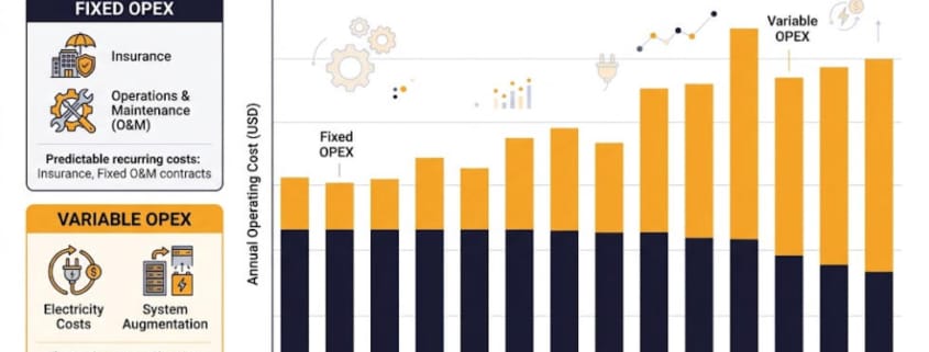
BESS OPEX splits into fixed costs and variable costs. Fixed costs include site lease, insurance, base O&M, and software.
Variable costs include charging electricity and performance-based O&M. An operating-cost model sums these items by year and feeds them into LCOS and cash-flow calculations.
CAPEX tells you what a system costs to build. OPEX tells you what it costs to run.
Two projects with similar CAPEX can still have very different LCOS, because O&M strategy or electricity price differs.
In a basic LCOS model, lifetime cost starts with initial CAPEX. Then add annual OPEX over the project life, plus charging cost, minus any residual value at the end.
Since BESS OPEX recurs every year, small fee changes can shift LCOS by tens of dollars per MWh. For deeper background, see our CAPEX vs LCOS guide and our BESS CAPEX calculation guide.
Fixed vs Variable BESS OPEX
Most BESS operating cost models split expenses into two buckets: fixed and variable.
Fixed OPEX
Fixed costs occur every year. This holds no matter how much the battery cycles.
Typical items include site lease and property taxes. For example, insurance and a base O&M contract count, along with a software subscription.
Security and site-management overhead round out fixed OPEX. This bucket often appears as dollars per kW-year, or as a flat sum per site per year.
Variable OPEX
Variable costs change with how the system runs. They include charging electricity, performance-based O&M fees, and degradation-related costs like augmentation.
Depending on the market and tariff structure, network charges, taxes, or other fees may also vary with imported energy, exported energy, throughput, or revenue. Variable OPEX usually appears as dollars per MWh charged or discharged.
A robust BESS OPEX model tracks fixed and variable costs separately. That way, you can test operating strategies without rebuilding the base cost structure each time.
Key BESS OPEX Components to Track
Use this checklist when you build an annual BESS OPEX model.
Operations and Maintenance (O&M)
O&M covers preventive maintenance, corrective repairs, remote monitoring, spare parts, and labor.
O&M contracts commonly take one of three forms: a fixed annual fee; a base fee plus a throughput-based charge; or a performance-linked arrangement with availability guarantees, incentives, and/or penalties.
Before signing, check what the contract covers. Monitoring, firmware updates, and cybersecurity patches usually make the list.
Major component replacement and grid-compliance upgrades usually don’t.
Charging Electricity Cost
Charging electricity is often the largest variable OPEX line. It depends on annual energy charged and round-trip efficiency.
Local tariffs matter too. Time-of-use pricing and solar co-location both move this number.
Include auxiliary consumption where possible. HVAC, pumps, controls, fire-safety systems, and standby loads can reduce net delivered energy or increase the energy purchased to support the system.
A simple estimate multiplies annual energy charged by average price. More advanced BESS OPEX models split charging by time block or market product, such as arbitrage or ancillary services.
Degradation, Augmentation, and Replacement
Degradation is another central consideration. Battery capacity fades over time, which cuts available energy, contracted performance, and lifetime throughput.
Since lower throughput drives LCOS up, projects manage this in a few ways: oversizing the battery upfront, adding augmentation later, or replacing parts of the system mid-life.
Once usable capacity drops below a threshold, augmentation usually kicks in. Projects usually model augmentation and major mid-life replacements as scheduled future CAPEX or replacement-CAPEX events.
For a simplified operating-cost budget, some teams show them alongside annual OPEX. But they should remain separate from routine O&M, and clearly appear in the year the expenditure occurs.
Insurance, Taxes, and Site Costs
Insurance and site costs matter too, especially for commercial and industrial projects. Typical items include property insurance, liability cover, and site security.
Some of these costs scale with CAPEX value. Others stay fixed per site.
Software, Data, and Compliance
Modern BESS also run on software. Energy management, market bidding, compliance reporting, and cybersecurity monitoring all count here.
Costs include license fees, per-site charges, and optional optimization modules. Some markets also require compliance audits, which adds a further OPEX line, as the U.S. Department of Energy’s storage program materials note.
A Simple BESS OPEX Model Structure
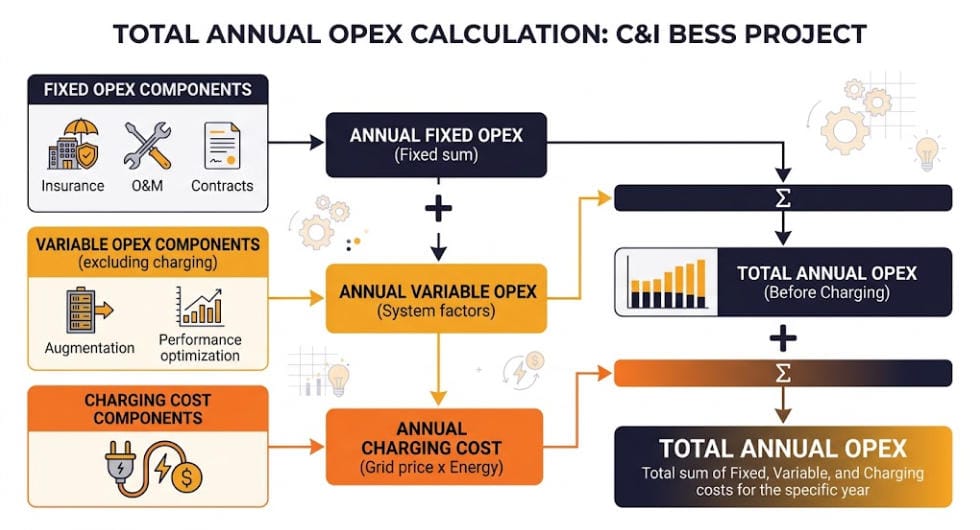
A basic annual operating-cost model sums three recurring lines: fixed OPEX, variable OPEX, and charging cost. The model tracks augmentation or replacement CAPEX separately, in the year it occurs.
Operating Costt = Fixed OPEXt + Variable OPEXt + Charging Costt
Lifecycle Spendt = Operating Costt + Augmentation/Replacement CAPEXt
Here, t is the operating year. Fixed OPEX covers recurring site, insurance, software, and contracted O&M costs. Variable OPEX changes with throughput or performance. Charging cost reflects the energy purchased to charge the system. Augmentation or replacement CAPEX appears only in years when the project needs it.
For LCOS or NPV work, discount each year’s total to present value at your chosen rate.
Worked Example: Annual BESS OPEX for a 2 MWh C&I System
For example, take a 2 MWh, 1 MW commercial and industrial system. Assume 250 equivalent full cycles per year and 90% round-trip efficiency.
Annual discharged energy: 2 MWh × 250 × 0.90 = 450 MWh/year
Annual charging energy: 450 MWh ÷ 0.90 = 500 MWh/year
At $2 per MWh discharged, throughput-based O&M is 450 × $2 = $900 per year. At $40 per MWh charged, annual charging electricity cost is 500 × $40 = $20,000.
Fixed OPEX is $18,000/year. Adding $900/year of throughput-based O&M and $20,000/year of charging electricity produces recurring operating cost of $38,900/year.
In year eight, the plan adds a $60,000 augmentation allowance as a separate capital expenditure, bringing that year’s total lifecycle spend to $98,900.
| Cost Line | Basis | Cost |
| Fixed OPEX | Lease, insurance, base O&M, software | $18,000/year |
| Variable O&M | 450 MWh discharged × $2/MWh | $900/year |
| Charging electricity | 500 MWh charged × $40/MWh | $20,000/year |
| Recurring operating cost | Years 1–7, excluding augmentation | $38,900/year |
| Augmentation/replacement CAPEX | Year 8 planning allowance | $60,000 |
| Lifecycle spend in Year 8 | Recurring operating cost + augmentation | $98,900 |
In a financial model, the $38,900 is recurring annual operating cost. However, you should normally model the $60,000 augmentation allowance as a separate future capital expenditure in Year 8.
This is a simplified example. Real models add escalation rates, more granular operating profiles, and often a revenue-side view too.
How BESS OPEX Feeds into LCOS and Project Decisions
BESS OPEX shapes LCOS two ways. First, it adds directly to lifetime cost: higher fees, pricier contracts, or costlier charging all push LCOS up.
Second, it shapes strategy indirectly. Expensive charging can push a project to cycle less, which then trims revenue too.
Before you commit to a BESS design, ask a few questions: what does fixed OPEX run per kW or per site, and how do contracts price variable O&M?
What charging strategy does the LCOS model assume, and how is degradation handled? Are software and compliance costs included?
Operating cost is only one side of BESS economics. To understand the revenue and avoided-cost opportunities that OPEX must be weighed against, see our BESS revenue streams and value-stacking guide.
Our Cost of Storing Energy guide walks through how these pieces combine into a full LCOS figure.
Operating cost is only one side of BESS economics. To understand the revenue and avoided-cost opportunities that OPEX must be weighed against, see our BESS revenue streams and value-stacking guide.
Frequently Aske d Questions
What Is a Typical BESS OPEX Range?
OPEX ranges vary by project type, region, and contract structure. Early-stage models sometimes use a provisional fixed O&M allowance of roughly one to three percent of initial CAPEX per year.
This is only a screening assumption, not a universal BESS benchmark. However, actual costs depend on system size, service scope, warranty coverage, cycling duty, labor rates, insurance, cybersecurity, site access, and whether the budget separates out major replacements.
Is Charging Electricity Cost Part of OPEX or LCOS Only?
Charging cost sits in both buckets. It is a recurring operating expense in cash-flow models, and a core input to LCOS.
However, in behind-the-meter projects, demand-charge savings can partly offset it. Self-consumed solar helps too.
How Do You Model Battery Degradation in OPEX?
Degradation itself is not a cash cost, but its effects are. Models capture it through lower available energy over time.
Also, augmentation or replacement spend in specific years counts, along with possible penalties when a project misses performance guarantees.
Together, these effects raise LCOS, because lower throughput and occasional large mid-life spending both add real cost over time.
Further Reading
- BESS CAPEX Calculation: How to Build the Total Investment Cost
- CAPEX vs LCOS: What BESS Cost per kWh Really Means
- Cost of Storing Energy: BESS LCOS Calculator Guide
- The Economics of BESS: Calculate ROI for Your Energy Storage
- Understanding BESS Specifications: The Complete 2026 Guide
- U.S. Department of Energy, Office of Electricity: energy storage program overview
BESS CAPEX Calculation: How to Build the Total Investment Cost
A BESS CAPEX calculation estimates the total investment to develop, procure, install, connect, and commission a battery storage system. Some costs scale with energy capacity, some scale with power capacity, and others are fixed or site-specific. Vendors often quote one dollar-per-kWh price. But that price hides several cost layers. Knowing those layers helps you check a quote. It also helps you build your own model or compare bids fairly.
| Quick Answer A BESS CAPEX calculation adds core costs, like battery, power conversion, and HVAC gear, to project costs, like installation, grid connection, and permits. It multiplies that combined per-kWh figure by system size. An escalation factor then adjusts the result for timing, giving total CAPEX. |
What Is a BESS CAPEX Calculation?
A BESS CAPEX calculation builds one investment figure for a battery project. Models use this figure as the Year-0 cost, the initial investment entered at the start of a project cash-flow, ROI, or LCOS model. In practice, getting the cost layers right beats chasing one flashy headline number.
Core System Costs
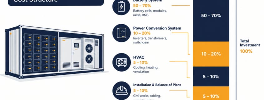
Core costs cover the technical parts of a BESS. These include the battery cells, the power conversion system, and the energy management system. They also include HVAC and fire safety gear, plus labor to put it all together. Together, these form one base cost per kWh, and they usually make up the largest share of a BESS CAPEX calculation.
- Battery cells and modules
- Power conversion system
- Energy management system
- HVAC and fire safety systems
- System integration labor and parts
Extra Project Costs That Add to CAPEX
A BESS needs more than hardware to become a real project. For example, install labor turns equipment into a working system, and grid connection work links the site to the utility. Project work also covers permits, site studies, and design, while a backup budget covers cost overruns. Skipping these costs is a common way a BESS CAPEX calculation ends up too low.
- Installation and EPC labor
- Grid connection work
- Project development work
- Contingency allowance
CAPEX Scope Checklist
Before comparing quotes, define what the CAPEX figure includes, since a BESS CAPEX calculation is only as accurate as its scope. A BESS proposal may be equipment-only, supply-and-install, EPC turnkey, or fully operational at the point of interconnection. A complete project scope may include:
- Battery cells, modules, racks, containers, and battery management systems (BMS)
- Power conversion system (PCS), transformer, switchgear, protection, SCADA, and communications
- Thermal management, fire detection, fire suppression or mitigation equipment where required, and auxiliary power
- Civil works, foundations, drainage, access roads, fencing, and site security
- Freight, commissioning, performance testing, and spare parts
- Engineering, procurement, construction, development, permitting, and studies
- Grid interconnection, network studies, metering, and utility upgrades
- Contingency, insurance during construction, and financing-related costs
Always state whether a quote is equipment-only, ex-works, delivered-duty-paid, supply-and-install, or turnkey EPC. A low per-kWh quote can leave out interconnection, civil works, commissioning, warranty extensions, or augmentation.
| Scope note Always compare quotes on the same delivery basis. An equipment-only price cannot be compared directly with a turnkey EPC price unless you add the omitted engineering, logistics, civil works, installation, commissioning, interconnection, contingency, and owner’s-cost items. |
The BESS CAPEX Calculation Formula
Once you know both cost layers, a basic BESS CAPEX calculation stays simple. First, add core costs to extra costs. Then multiply that combined per-kWh figure by system size.
| Base CAPEX = (Core Costs + Extra Costs) × Size (kWh) |
Separate Power and Energy Costs for a Realistic Model
A single dollar-per-kWh figure works for an early estimate. But real BESS cost depends on both energy size and power size, because PCS, transformers, and switchgear scale with power, not just energy. As a result, this version of a BESS CAPEX calculation gives a more realistic figure for larger or longer-duration systems.
| Base CAPEX = (Cₑ × E) + (Cₚ × P) + Fixed Costs + Site Costs |
- Cₑ = energy cost, in $/kWh
- E = usable or installed energy, in kWh
- Cₚ = power cost, in $/kW
- P = rated AC power, in kW
- Fixed costs = items that don’t scale with size
- Site costs = civil works and grid connection
For example, this split matters most when you compare a 2-hour system and a 4-hour system at the same power rating. Battery cost changes a lot between them, while PCS and grid connection cost often do not.
Account for Escalation and Timing
A cost estimate ties to a base date. But a project often gets built later, and prices for gear, labor, and site work can shift in that gap. Because of this, a complete BESS CAPEX calculation has to account for timing, not just today’s prices.
| Escalation Amount = Base CAPEX × Escalation Rate Total CAPEX = Base CAPEX × (1 + Escalation Rate) |
Here, the escalation rate is the expected cost shift from the estimate date to the build date. For example, if base CAPEX runs $540,000 and the escalation rate runs 4 percent, total CAPEX comes to $561,600.
For a multi-year build, model escalation by cost category and year instead of one flat rate.
| Total CAPEX (Year t) = Base CAPEX × (1 + Escalation Rate)^t |
Round the final figure to whole dollars for reporting.
| Escalation vs. Contingency Escalation reflects expected future price changes between the cost-estimate date and the purchase or construction date. Contingency covers uncertainty and execution risk in the defined scope. A robust BESS CAPEX model may include both, but they should be tracked as separate line items. |
Worked Example: BESS CAPEX Calculation for a 2 MWh System
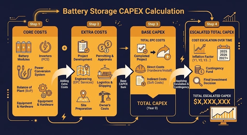
The steps below walk through a full BESS CAPEX calculation from start to finish. First, though, in a real estimate, state whether the energy figure means nominal battery energy, usable energy at the start of life, or AC-deliverable energy at the connection point. Otherwise, the definition changes the per-kWh result and the fairness of any quote comparison.
Assume a 2 MWh battery project with these numbers. Size runs 2,000 kWh. Core cost runs $210 per kWh. Extra cost runs $60 per kWh. Escalation rate runs 4 percent, for a one-year build.
Step 1: Base cost per kWh. Add $210 and $60. That gives $270 per kWh.
Step 2: Base CAPEX. Multiply $270 by 2,000 kWh. That gives $540,000.
Step 3: Escalation amount. Multiply $540,000 by 4 percent. That gives $21,600.
Step 4: Total CAPEX. Multiply $540,000 by 1.04. That gives $561,600.
| Input | Value |
| Nominal system energy | 2,000 kWh |
| Core system cost | $210/kWh |
| Project/site cost | $60/kWh |
| Base CAPEX | $540,000 |
| Escalation allowance | 4% |
| Escalation amount | $21,600 |
| Total CAPEX | $561,600 |
| Implied total CAPEX | $280.80/kWh |
This is an early-stage estimate only. It does not set a market price for a specific system or site.
This method is best for screening and early-stage budgeting. As the project advances, replace generic per-kWh assumptions with supplier quotes, site-specific civil estimates, interconnection studies, construction schedules, and a defined EPC scope.
What This CAPEX Number Doesn’t Tell You
A BESS CAPEX calculation is only the first half of the cost picture. It shows the cost to develop, procure, and build a system within a defined scope, but it does not show the cost of owning and operating the system or the value it creates.
For the recurring costs that sit outside Year-0 CAPEX — including O&M, charging electricity, insurance, software, and degradation-related spending — see our BESS OPEX and operating cost model.
Instead, financing costs, O&M, charging energy, degradation, augmentation, revenue, and demand-charge savings belong in an LCOS, operating-cost, or project-ROI model.
Depending on project scope, land, permitting, development, and interconnection expenses may be included in CAPEX or tracked separately.
CAPEX shows the cost to build the asset, not the value it can create through arbitrage, demand-charge savings, capacity payments, or grid services. Explore these opportunities in our BESS revenue streams and value-stacking guide.
For the full cost picture, pair this figure with an LCOS model. Our CAPEX vs LCOS guide explains why these two numbers differ. It also covers 2025-2026 price benchmarks. Our LCOS Calculator Guide walks through the full cost formula step by step.
The U.S. Department of Energy tracks storage cost trends through its energy program. Its guidance uses a similar cost-layer approach to the one here.
Frequently Asked Questions
How Accurate Is a BESS CAPEX Calculation Without a Vendor Quote?
A calculation built from industry ranges gives a fair early estimate. But a vendor quote reflects real gear prices and site conditions. Use the calculation for early planning. Then refine it once quotes come in.
Does BESS CAPEX Include Land and Permitting Costs?
It depends on the project scope and the delivery basis used in the quote. Some models include land, permitting, development, owner’s engineering, and interconnection in CAPEX. Others track some or all of these costs separately. So, before comparing figures, confirm exactly which items are included, excluded, or treated as allowances in your BESS CAPEX calculation.
How Often Should You Re-Run a BESS CAPEX Calculation?
Re-run the BESS CAPEX calculation any time a big input changes. New vendor prices, a new timeline, or a new escalation rate can all shift total CAPEX. As a result, many teams re-check CAPEX at each project milestone.
Further Reading
CAPEX vs LCOS: What BESS Cost per kWh Really Means
Cost of Storing Energy: BESS LCOS Calculator Guide
The Economics of BESS: Calculate ROI for Your Energy Storage
Understanding BESS Specifications: The Complete 2026 Guide
U.S. Department of Energy, Office of Electricity: energy storage program overview
CAPEX vs LCOS: The BESS Cost Trap
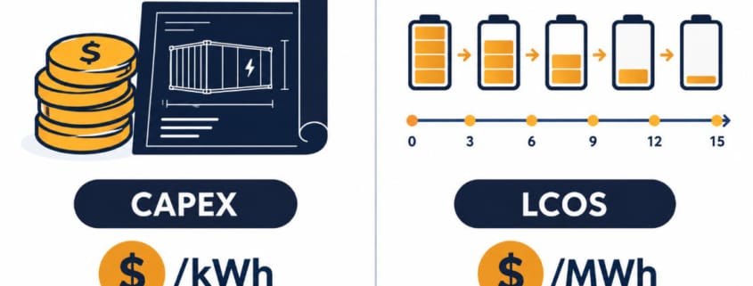
BESS CAPEX vs LCOS confusion causes real problems. It shows up whenever you compare storage quotes. CAPEX tells you what a system costs to build. LCOS, however, tells you the lifetime cost of each kWh it delivers. A project with attractive upfront CAPEX can still show a materially higher LCOS. This happens because it cycles infrequently, degrades faster than expected, or charges from expensive electricity.
| Quick Answer CAPEX and LCOS are different BESS cost metrics. CAPEX is the upfront installed cost per unit of battery capacity, commonly expressed in $/kWh. LCOS is the lifetime cost per unit of electricity discharged, commonly expressed in $/MWh or $/kWh delivered. For example, $65–$150/MWh equals $0.065–$0.150/kWh of delivered energy. |
Why CAPEX vs LCOS Gets Confused
Vendors, developers, and investors often use “cost per kWh” loosely. Sometimes they mean CAPEX. Sometimes they mean LCOS. In short, the two numbers measure very different things.
First, CAPEX ($/kWh) is simple. It is the upfront cost to install one kWh of storage. It covers battery cells, the power conversion system, balance of system, and EPC work.
LCOS ($/kWh or $/MWh), by contrast, works differently. It is the lifetime cost of each kWh the system actually discharges. It folds in CAPEX, O&M, charging electricity, efficiency losses, and degradation.
To see how annual O&M, charging cost, insurance, software, and future augmentation are modeled, read our BESS OPEX and operating cost model.
Mixing up CAPEX vs LCOS leads to bad comparisons. For instance, a system with low CAPEX can still post a high LCOS. This happens because it cycles rarely, degrades fast, or charges from costly power.
Which one should you use? Use CAPEX to compare build costs. Then use LCOS to compare long-term value. For a full LCOS walkthrough with formulas and worked examples, see our Cost of Storing Energy: BESS LCOS Calculator Guide.
To build an early-stage installed-cost estimate before comparing it with LCOS, see our BESS CAPEX calculation guide.
2025–2026 BESS Cost Benchmarks
Recent industry cost benchmarking gives a useful reality check for 2026 budgeting and LCOS modeling.
However, these are directional market benchmarks, not vendor-quote substitutes. Scope varies by duration, geography, delivery terms, inclusion of EPC and interconnection, tax treatment, warranty coverage, and augmentation assumptions.
Benchmark figures in this section reflect 2025–2026 industry analyses, including BloombergNEF, Ember, and Lazard reporting. Project-specific results may vary substantially by duration, location, operating profile, and procurement scope.
Utility-Scale CAPEX ($/kWh)
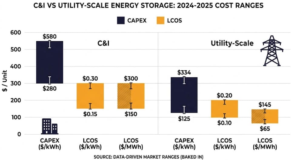
Global average turnkey BESS pricing landed near $117/kWh in 2025 (BloombergNEF, 2025). All-in 4-hour-plus utility projects outside the US and China, meanwhile, ran closer to $125/kWh in late 2025 (Ember, 2025). Utility-grade LFP cell prices sat around $55–$75/kWh. Full system costs run higher once PCS, balance of system, and EPC work get added.
C&I CAPEX ($/kWh)
Typical commercial and industrial installed costs run $250–$450/kWh, depending on duration, site complexity, and local balance-of-system costs. However, larger, standardized containerized C&I systems can fall toward $180–$300/kWh in favorable markets.
LCOS Benchmarks ($/MWh)
Well-sited 4-hour LFP projects often show an LCOS of $65–$150/MWh in 2025. The exact number depends on cycles, financing, and local electricity prices. Recent US utility-scale analysis, for example, covers unsubsidized 2-hour and 4-hour systems in 2026 (Lazard LCOS analysis, 2026). It points to a wider $210–$414/MWh range, varying by use case and region. These ranges show why context matters for BESS CAPEX vs LCOS comparisons. Once you factor in duration, cycles, and local costs, LCOS can shift by two to three times, even between projects with similar CAPEX.
The Simple BESS CAPEX vs LCOS Formula
For quick comparisons, use a simplified LCOS formula:
| LCOS ≈ Total Lifetime Costs ÷ Total Lifetime Energy Delivered |
Total Lifetime Costs equal CAPEX plus lifetime O&M plus lifetime charging cost, plus augmentation if needed, minus residual value.
Meanwhile, Total Lifetime Energy Delivered is every kWh discharged over the project life, after accounting for round-trip efficiency and degradation.
A more rigorous version discounts future costs and energy to present value. It also models degradation and augmentation explicitly. Discount rate matters here: a project with the same physical performance can show a higher LCOS when financing costs are higher, or when more of its usable energy arrives later in its life. You don’t need the full discounted formula for every conversation. But it’s the right mental model once you compare long-duration storage, different chemistries, or PPAs.
Worked Example: BESS CAPEX vs LCOS for a 1 MWh C&I System
Assume a 1 MWh, 2-hour C&I BESS with these simplified assumptions:
- CAPEX: $350,000 ($350/kWh)
- Life: 15 years
- Cycles: 250 per year
- Round-trip efficiency: 90%
- O&M: 1.5% of CAPEX per year (about $5,250/year)
- Average charging cost: $0.04/kWh
- No augmentation, no residual value
Step 1: Lifetime energy delivered. First, annual discharged energy comes to 1,000 kWh × 250 cycles × 0.90 efficiency, or 225,000 kWh per year. So, over 15 years, that totals 3,375,000 kWh.
Step 2: Lifetime costs. Next, add up the costs. CAPEX runs $350,000. Then O&M adds $78,750 over 15 years. Charging cost, once you account for the 90% efficiency, works out to about $150,000 over the same period. In total, lifetime cost lands near $578,750.
Step 3: Simple LCOS. Finally, divide $578,750 by 3,375,000 kWh. The result is roughly $0.17/kWh, or $171.5/MWh. That sits at the higher end of the C&I range, because fewer cycles and a higher installed cost pull it up.
Add battery degradation, such as 1.5% annual capacity fade, and lifetime energy falls. LCOS then rises. This is exactly why serious project models need to include degradation explicitly.
Instead of a full project-ROI model, this simplified example excludes financing, taxes, demand-charge savings, incentive value, replacement or augmentation, downtime, and end-of-life value. It illustrates LCOS only. LCOS tells you the cost of delivered stored electricity. It doesn’t by itself show whether demand-charge reduction, resilience, capacity payments, or ancillary-service revenue makes a C&I system profitable.
How to Lower Your LCOS
A handful of levers consistently pull LCOS down, regardless of chemistry or vendor:
- Increase effective cycles. Align operation with price signals so the battery cycles more often without excess degradation.
- Extend duration where it makes sense. For example, spreading CAPEX over more MWh often lowers LCOS, especially for 2 to 4-hour systems.
- Reduce charging cost. Instead, use time-of-use arbitrage, renewable co-location, or PPAs to lower the average price of the electricity you charge with.
- Choose low-degradation designs. LFP chemistry and strong thermal management, such as liquid cooling, help sustain throughput over 10 to 15-plus years. Since duration and C-rate choices drive this trade-off too, see our BESS C-Rate guide for how sizing affects cost and cycle life.
- Standardize BOS and EPC. Containerized, repeatable designs cut soft costs and installation risk, especially across multi-site C&I portfolios.
C&I vs Utility: BESS CAPEX vs LCOS Compared
| Aspect | C&I BESS | Utility-Scale BESS |
|---|---|---|
| Typical duration | 1–4 hours | 2–6+ hours |
| Main use cases | Demand charge reduction, backup, limited arbitrage | Renewable firming, capacity, ancillary services, arbitrage |
| Installed CAPEX | ~$250–$450/kWh (as low as $180–$300/kWh for large standardized systems) | ~$117–$125/kWh in selected global 4-hour-plus utility-scale benchmarks (2025); project quotes vary by region and scope |
| Cycles per year | Often 150–300 | Often 300–700+, depending on market |
| Typical LCOS | ~$150–$250/MWh, highly site-specific | ~$65–$150/MWh for well-sited 4-hour LFP; higher for shorter duration or costly regions |
| Primary value driver | Demand-charge management, resilience, tariff optimization, behind-the-meter value | Capacity, wholesale arbitrage, ancillary services, renewable integration |
The pattern is consistent: because C&I projects usually carry higher CAPEX and run fewer cycles, LCOS lands higher per MWh than a utility project. However, that doesn’t make them worse investments. Instead, value comes from demand charge savings, resilience, and local grid services, not from LCOS alone.
What to Ask Your BESS Vendor
Move past headline dollar-per-kWh numbers by, instead, asking vendors and EPCs:
- What cycle profile, in cycles per year, depth of discharge, and C-rate, sits behind your cost and performance claims?
- What degradation warranty do you offer, such as percent capacity remaining after 10 years at a stated cycle rate?
- How do you model round-trip efficiency and auxiliary loads in your LCOS or yield estimates?
- Which CAPEX components are included: cells, PCS, balance of system, EPC, interconnection, commissioning, O&M?
- Can you provide an LCOS or cash-flow model with sensitivity to electricity price, cycles, and degradation?
Our BESS specifications guide walks through the datasheet numbers behind these questions. Because of that, it helps you compare vendor quotes on equal terms, not just a single headline figure. In practice, these questions push the conversation past upfront cost. They put it on a consistent, lifetime-value basis instead.
Frequently Asked Questions
Why Does BESS CAPEX vs LCOS Matter for My Project?
CAPEX only tells you what a system costs to build. LCOS, however, tells you what it actually costs to run over its life. Because of this, a project decision based on CAPEX alone can miss a system that costs less per kWh delivered over 15 years.
Is a Lower CAPEX Always Better for BESS?
Not necessarily. A lower-CAPEX system can still post a higher LCOS. Poor cycle life, fast degradation, or low efficiency can all cause this. So, always weigh CAPEX together with expected cycles, degradation, and O&M.
What Is a Good LCOS for BESS in 2026?
It depends on your market and use case. Well-sited 4-hour utility LFP projects commonly land around $65–$150/MWh in current industry benchmarking. C&I projects often sit higher, because fewer cycles and higher installed cost drive that gap. Even so, demand charge savings and resilience can still make them attractive.
How Does Degradation Affect BESS Cost Over Time?
Degradation shrinks the total energy a battery can deliver over its life. Because of that, LCOS rises if CAPEX and other costs hold steady. Even 1–2% annual capacity fade, for example, can meaningfully change your cost per kWh and your payback period.
A lower LCOS does not automatically mean a stronger investment case. Project returns also depend on revenue and avoided-cost opportunities; see our BESS revenue streams and value-stacking guide.
Further Reading
- Cost of Storing Energy: BESS LCOS Calculator Guide
- BESS C-Rate: How Charge, Discharge Rate & Price Are Linked
- Understanding BESS Specifications: The Complete 2026 Guide
- The Economics of BESS: Calculate ROI for Your Energy Storage
- U.S. Department of Energy, Office of Electricity: energy storage program overview
Types of BESS by Application: A Complete Guide
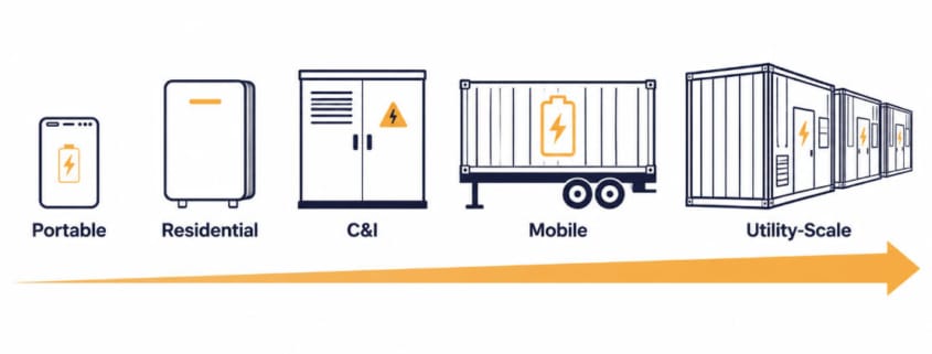
You’ll find battery energy storage systems, or BESS, in settings ranging from portable power and rooftop solar homes to factories, construction sites, and grid-scale renewable projects. These systems all store and deliver electricity, but the types of BESS available differ substantially in size, packaging, controls, safety design, and grid connection.
First, matching the right type of BESS to your project starts with knowing what each one is built for.
| Quick Answer The five common types of BESS by application are portable, residential, C&I, mobile, and utility-scale. They range from compact systems storing watt-hours or a few kilowatt-hours to grid-connected projects storing hundreds of megawatt-hours. |
BESS can also be classified by battery chemistry, system configuration, duration, or grid position. This guide focuses specifically on types of BESS by application — where the system is used and what it is designed to do.
Why There Are Different Types of BESS
Most rechargeable BESS combine batteries with monitoring and protection, power electronics, and thermal-control or enclosure features. But the exact architecture varies by size and application.
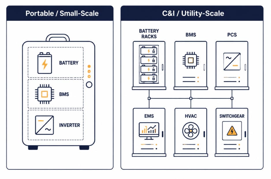
A portable power station often integrates these functions into one product. C&I and utility-scale projects, on the other hand, typically use dedicated subsystems instead: battery racks, a battery management system (BMS), a power conversion system (PCS), HVAC, fire protection, transformers, switchgear, and site controls.
An energy management system (EMS) is a separate, functional layer, not something that simply switches on above a size threshold. It coordinates charging and discharging according to site objectives, such as solar self-consumption, tariff optimization, backup reserve, generator reduction, or grid-service dispatch.
Large C&I and utility-scale projects generally require a dedicated EMS or site controller. Residential and portable products, meanwhile, often provide simpler embedded control functions instead. The underlying logic is similar; it’s just running at a smaller scale.
A few factors drive which type of BESS fits a given project:
- How much power and energy the application needs, and for how long
- What the system is trying to achieve — backup power, solar self-consumption, peak shaving, demand-charge reduction, generator reduction, energy arbitrage, or grid services
- Whether the system stays in one place or moves
- How it connects to the grid, and at what voltage level
- What safety and compliance standards apply at that scale
Because of these differences, BESS spans a huge range. It ranges from a compact power station to a utility-scale installation that can occupy a large, purpose-designed site. For the full picture on how each type is built, see our complete guide to battery energy storage systems.
The 5 Types of BESS by Application
1. Portable BESS
Portable battery energy storage systems are compact, self-contained units built for power on the go. They typically range from a few hundred watt-hours to a few kilowatt-hours. Because they are small and easy to carry, they suit camping, remote work, field operations, and emergency response where power is needed without a permanent installation.
Most current portable power stations use lithium-ion cells, often lithium iron phosphate (LFP), because they offer a practical balance of energy density, cycle life, and safety characteristics. They typically combine the battery, inverter/charger, protection functions, and user controls in one enclosure rather than using a separate, dedicated PCS.
Portable units commonly include battery monitoring, protection, and temperature sensing. Unlike larger stationary systems, they generally do not require dedicated HVAC equipment or liquid-cooling loops.
They usually rely on embedded controls rather than a separate site-level EMS. Depending on the product, these controls may manage charging sources, output limits, backup behavior, or simple scheduling. The exact control and thermal design varies by product and power rating.
Learn more in our guide to portable battery energy storage systems — one of the lightest types of BESS covered in this guide.
2. Residential BESS
Home energy storage systems pair with rooftop solar to store excess daytime generation for evening use. Most residential systems run roughly 5-20 kWh. Larger systems, though, serve high-load homes, EV charging, electrified heating and cooling, or longer backup requirements.
In practice, the right size for a given household depends on its load profile, solar output, desired backup circuits, and target backup duration.
Installers commonly mount residential BESS units on a wall or floor. They connect through a hybrid inverter or a separate battery inverter, depending on the solar and electrical design, and include battery monitoring, protection, and thermal-control features built for long-term stationary operation.
Many also use energy-management logic for solar self-consumption, tariff optimization, backup reserve settings, or EV charging coordination. That’s a simpler, embedded version of the dispatch control found in larger C&I and utility-scale systems.
See our guide on what a home energy storage system is for a full breakdown of this type of BESS.
3. Commercial & Industrial (C&I) BESS
C&I battery energy storage systems serve businesses, factories, and campuses that want to cut demand charges, add backup resilience, or pair storage with on-site renewables. These systems generally range from tens of kilowatt-hours to several megawatt-hours.
Engineers often specify these systems by both power and duration — for example, 500 kW / 1 MWh or 2 MW / 4 MWh. That’s because a site’s peak load, tariff structure, backup requirement, and renewable-generation profile all shape the right configuration.
At this scale, however, design gets more involved. C&I systems typically need dedicated enclosures, active thermal management, and integration with a facility’s existing electrical infrastructure.
Depending on the site and jurisdiction, the design may include fire detection and suppression, emergency shutdown, HVAC or ventilation, electrical isolation and protection, access control, and remote monitoring.
We cover this application in depth across our C&I BESS series, starting with key components in C&I BESS — one of the most widely deployed types of BESS today.
4. Mobile BESS
Mobile battery energy storage systems are trailer-mounted or containerized units that travel to wherever power is needed. That could mean a construction site, an event venue, a disaster response zone, or temporary grid support during planned outages.
Mobile BESS is often deployed alongside temporary grid connections, renewable generation, or diesel generators. In hybrid power setups, the battery can reduce generator runtime and improve generator loading efficiency.
It can also cover short-duration peak power. This is often the real economic case for choosing a mobile unit over a standard fixed C&I system.
Because they need to move, mobile units prioritize a rugged, self-contained design. They pack the battery, BMS, PCS, and often a built-in cooling system into a single towable or shippable unit. That trades some of the customization of a fixed installation for flexibility.
Learn more in our guide to mobile BESS, a uniquely flexible type of BESS built for temporary deployments.
5. Utility-Scale BESS
Utility-scale battery energy storage systems are the largest deployment type, ranging from several megawatt-hours to hundreds of megawatt-hours. They commonly use containerized or modular outdoor enclosures, combined with separate PCS, transformer, switchgear, protection, and control equipment.
The final layout depends on project capacity, duration, climate, fire-safety design, grid interconnection, and site constraints. So while containerized designs are common, they aren’t universal.
As a result, utilities, developers, and independent power producers deploy utility-scale BESS for frequency regulation, renewable-energy shifting and firming, capacity support, peak management, energy arbitrage, and other grid services.
Because of their size, these projects typically require detailed interconnection studies, protection coordination, dedicated switchgear, and coordination with the relevant grid operator. See the U.S. Department of Energy’s overview of grid-scale energy storage for more on how these systems support the wider grid. Utility-scale projects may connect at either distribution or transmission voltage, depending on the project’s rating.
Read our complete guide to utility-scale BESS, the largest of the five types of BESS by application, for the full picture.
Comparing BESS Types by Application
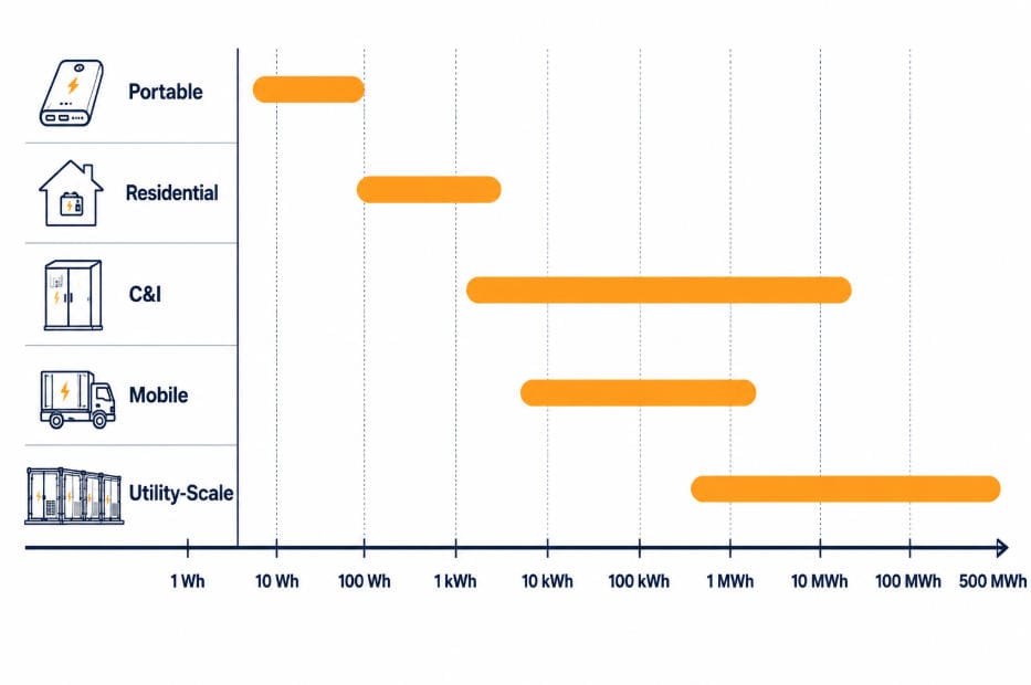
| Type | Typical Energy Capacity | Mobility | Primary Use Case |
|---|---|---|---|
| Portable BESS | A few hundred Wh to a few kWh | Fully mobile, carry-anywhere | On-the-go power, camping, remote work |
| Residential BESS | 5-20 kWh (larger for high-load homes) | Fixed installation | Solar storage, evening/overnight household use |
| C&I BESS | Tens of kWh to several MWh | Fixed installation | Demand charge reduction, backup, renewable pairing |
| Mobile BESS | Tens of kWh to a few MWh | Trailer-mounted or containerized, transportable | Construction sites, events, disaster response, temporary grid support |
| Utility-Scale BESS | Several MWh to hundreds of MWh | Fixed, commonly containerized/modular | Frequency regulation, capacity firming, grid-scale renewable integration |
Energy capacity indicates how much electricity a system can store. Power rating, expressed in kW or MW, determines how quickly it can charge or discharge.
How to Choose the Right Type of BESS
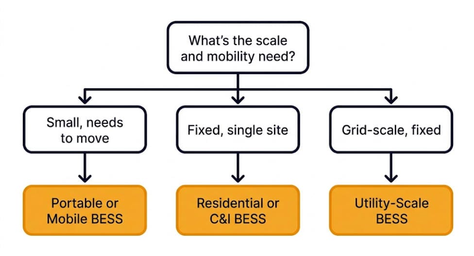
Picking the right type of BESS comes down to matching the system to the application:
- Power and energy requirement — determine the kW/MW rating, the usable kWh/MWh capacity, and the required discharge duration. Their relationship matters: a 1 MW / 2 MWh system, for example, is built for about two hours of discharge at rated power, before accounting for operating limits and degradation.
- Operating objective — solar self-consumption, peak shaving, backup power, generator reduction, arbitrage, or grid services each call for different controls and designs.
- Mobility and site constraints — decide whether the system needs to be fixed, trailer-mounted, transportable, indoor, outdoor, containerized, or modular.
- Grid connection and operating mode — systems may run off-grid, behind the meter, in a microgrid, or front of meter. Larger projects may interconnect at distribution or transmission level, depending on their power rating and local grid requirements.
- Safety, permitting, and compliance — requirements vary by jurisdiction, installation location, fire strategy, electrical design, and project scale.
- Budget and delivery timeline — factor in civil works, interconnection, switchgear, installation, commissioning, and ongoing operations and maintenance, not just equipment cost.
For most first-time buyers, matching the application to one of the five categories above is the fastest way to narrow down the right BESS type. Once that’s settled, these six factors help define the exact specification.
Conclusion
The right type of BESS depends first on the application. That means how much power and energy are needed, how long the system must operate, whether it needs to move, and how it will connect to the site or grid.
In general, portable and residential systems prioritize simplicity and compact design. C&I and mobile systems, meanwhile, balance resilience, flexibility, and site economics. Utility-scale projects, by contrast, are engineered for grid integration and large-scale dispatch.
Once you’ve identified the right application category, the next step is to define the required power rating, usable capacity, duration, site conditions, safety requirements, and control strategy. For a broader technical overview, see our complete guide to battery energy storage systems.
Frequently Asked Questions
What are the main types of BESS?
The main types of BESS by application are portable, residential, commercial and industrial (C&I), mobile, and utility-scale. Each one fits a different setting, from a few hundred watt-hours to hundreds of megawatt-hours.
What is the difference between a BESS and a battery?
In short, a battery is the electrochemical storage component. A BESS, however, is the complete system built around batteries, including battery monitoring and protection, power conversion, controls, thermal management, enclosure equipment, and — in larger projects — site-level safety and grid-interconnection equipment.
How are BESS systems classified besides application?
BESS can also be classified by battery chemistry, such as LFP or NMC. Other common classifications include system configuration (AC-coupled or DC-coupled), duration, mobility, and whether it operates behind the meter or front of meter. This guide classifies BESS by its end-use application.
What Size Should This Type of BESS Be for My Home?
Most residential systems run roughly 5-20 kWh. Larger systems, though, serve high-load homes, EV charging, or longer backup requirements — the right size depends on your household’s load profile, solar output, and desired backup circuits.
What’s the difference between C&I and utility-scale BESS?
C&I BESS typically ranges from tens of kilowatt-hours to several megawatt-hours, and serves a single business or facility. Utility-scale BESS is much larger, from several megawatt-hours to hundreds of megawatt-hours, and serves the broader grid instead of one site.
Which Types of BESS Can Be Moved Once Installed?
Fixed installations like residential, C&I, and utility-scale BESS generally don’t move once installed. Mobile BESS units are the exception — manufacturers build them specifically to be trailer-mounted or containerized for transport between sites.
Do all types of BESS use the same battery chemistry?
Most modern BESS across all five categories use lithium-ion batteries. Many new stationary systems use LFP chemistry because of its cycle-life and thermal-stability characteristics.
Chemistry can still affect system design, safety strategy, footprint, performance, and cost. However, this guide classifies BESS primarily by application, scale, packaging, and operating requirements.
Further Reading
The Cost of Stranded Capacity: What Poor BMS Design Costs BESS Asset Owners
BESS financial models assume throughput follows a clean degradation curve. Real fleets don’t behave that way. Stranded capacity is the gap between the two.
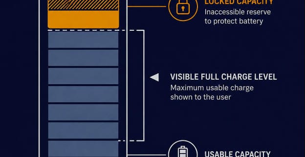
Every year, some capacity goes stranded. That’s capacity the pack technically still has, but the BMS can’t safely deliver it. Stranded capacity never shows up in a standard ROI model.
Our guide to calculating BESS ROI covers the standard model: capex, opex, revenue streams, payback period. This piece covers a value-at-risk category that model doesn’t capture.
Quick Answer
Stranded capacity is battery capacity a BESS has but can’t deliver, due to SOC drift, cell imbalance, or overly conservative cutoffs. It’s a hidden cause of revenue below projections. Fixing the underlying BMS design can recover real throughput — up to 10% in mid-to-late project life, in one internal analysis.
Key Takeaways
- Stranded capacity is real capacity the battery holds but the BMS can’t safely deliver. It’s a design and control issue, not a warranty defect or a safety problem by itself.
- One internal DCIR-adaptive cutoff analysis found up to 10% of effective throughput can be recovered in mid-to-late project life, just by replacing a fixed cutoff voltage with a DCIR-adaptive one.
- Cell imbalance alone can strand real energy. A pack stops charging or discharging when its weakest cell hits a limit, well before the rest of the pack is full or empty.
- SOC estimation drift compounds silently. Left uncorrected, it produces wrong dispatch decisions and wrong revenue forecasts, not just an inaccurate percentage on a screen.
- None of these issues show up in a standard BESS ROI model’s assumptions. Asset owners and EPCs who ask about them at the RFP or commissioning stage catch value a generic warranty review misses.
Why Stranded Capacity Doesn’t Show Up in a Standard ROI Model
This is a different problem from capacity stranded by deliberate oversizing. See our BESS oversizing guide for that scenario, where idle nameplate capacity is a sizing choice, not a BMS malfunction. The stranded capacity covered here comes from BMS design and control issues on capacity the system was never meant to leave unused.
A standard BESS ROI model tracks one degradation number: State of Health. It assumes capacity fades on a smooth, predictable curve, and revenue scales down with it.
That model misses a second category entirely. Stranded capacity isn’t capacity the battery has lost. It’s capacity the battery still has, that the BMS can’t reach.
Our own DCIR-adaptive cutoff design analysis found this gap directly. A fixed low-voltage cutoff is sized conservatively for a fresh pack.
It stops discharge earlier and earlier as internal resistance rises with age.
A liquid-cooled BESS cycle-life comparison echoes the same finding. A DCIR-adaptive cutoff can recover up to 10% of effective throughput in mid-to-late project life.
That’s real revenue a fixed-cutoff design leaves on the table, every single cycle.
What Stranded Capacity Actually Looks Like
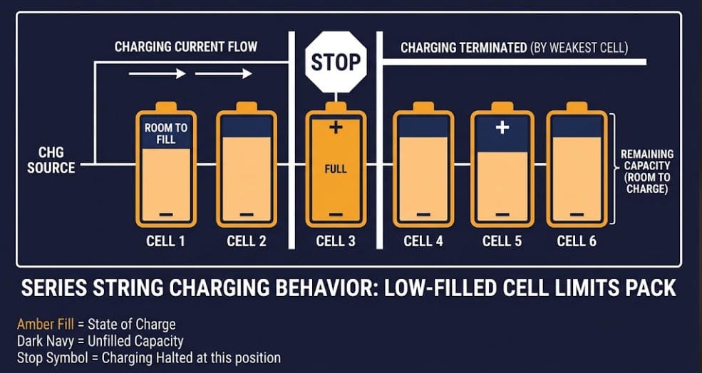
The mechanism is well documented in industry practice. Trade coverage of battery imbalance in BESS describes stranded energy this way: capacity that stays inaccessible because a small number of cells reach their limits first.
Charging can stop even though most of the pack still has room. Discharge can end while real energy still sits in the stronger cells.
Neither event trips an alarm. Neither shows up as a fault. The pack just quietly delivers less than it should, cycle after cycle.
Performance guarantees compound the problem. Industry analysis of BESS performance guarantees notes that a generic throughput guarantee often ignores which degradation mechanism actually applies.
Frequency regulation stresses a pack differently than energy shifting does.
A guarantee calibrated for the wrong use case can look satisfied on paper while stranded capacity quietly erodes real revenue underneath it.
Four Root Causes That Strand Throughput
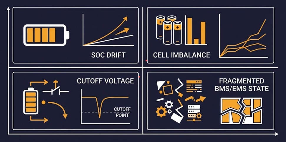
Stranded capacity has a small number of well-understood causes. Each one has a specific design fix, not just a monitoring dashboard.
SOC Estimation Drift
A BMS that only counts coulombs accumulates error every cycle, with no way to self-correct. Dispatch decisions built on a drifted SOC number are wrong, even when the battery itself is healthy.
This kind of drift is easy to miss because it doesn’t trigger any alarm. The dispatch software keeps making decisions confidently, just on the wrong number.
Over months, the gap between estimated and true state of charge can grow large enough to strand real capacity at both ends of the cycle — charge or discharge stopping based on a number that no longer matches reality.
See our EKF SOC estimation design guide for how a Kalman-filter-based estimator corrects for this instead of just counting and hoping.
In-Service Cell Imbalance
Cells drift apart in charge level over months of real-world cycling, even when they started out closely matched. The weakest cell then governs the whole string’s usable window.
Imbalance rarely announces itself either. Two cells built to the same spec can still diverge under real thermal and manufacturing variation, cycle after cycle.
Left uncorrected, that gap widens on its own. More of the pack’s true capacity quietly becomes capacity the BMS won’t touch.
See our in-service cell imbalance guide for how to detect and correct drift before it strands real capacity.
Premature Low-SOC Cutoffs
A fixed cutoff voltage, set conservatively for a brand-new pack, gets more conservative every year as internal resistance climbs. It ends discharge earlier than the chemistry actually requires.
The effect compounds quietly with age. A cutoff that was appropriately conservative in year one becomes needlessly conservative by year five, since resistance keeps climbing while the cutoff voltage stays fixed.
Nobody adjusts it, because nothing about the system looks broken. It just delivers a little less every year than it safely could.
See our DCIR-adaptive cutoff design guide for the design behind the 10% recovery figure cited above.
Fragmented BMS and EMS State
SOC, SOH, imbalance data, and cutoff logic often live in separate modules that don’t share state cleanly. Each module compensates conservatively for what it doesn’t know, and those safety margins stack up.
Each layer, acting alone, makes a reasonable decision. Stacked together, those decisions compound into capacity nobody intended to strand.
See our integrated BMS control architecture guide for how a shared-state design removes the guesswork each layer would otherwise carry on its own.
Root Causes, Symptoms, and Fixes at a Glance
The table below lines up all four causes of stranded capacity covered here, alongside how each one shows up and the design fix that addresses it.
| Root Cause | How It Shows Up | Design Fix |
| SOC estimation drift | Wrong dispatch decisions; inaccurate revenue forecasts | Kalman-filter-based SOC estimation with periodic recalibration |
| In-service cell imbalance | String stops early on charge or discharge | Active balancing tuned to LFP’s flat voltage curve |
| Premature low-SOC cutoffs | Discharge ends before chemistry limits are reached | DCIR-adaptive cutoff voltage, not a fixed one |
| Fragmented BMS/EMS state | Conservative margins stack across separate modules | Integrated, shared-state control architecture |
Translating Stranded Capacity Into Revenue Terms
A simple illustration makes the scale concrete. Consider a 10 MWh system earning a blended $80 per MWh-cycle across arbitrage and grid services, cycling roughly 300 times a year.
That works out to about $240,000 in annual gross revenue at full throughput.
If stranded capacity quietly removes 5% of usable throughput, roughly $12,000 in potential annual revenue never gets captured. Not because the battery lacks the energy — because the BMS won’t release it.
At the higher end of the up-to-10% figure cited earlier, that figure roughly doubles to about $24,000 a year.
These are illustrative figures, not a forecast for any specific project. Actual revenue per cycle and stranded-capacity percentage vary by market, duty cycle, and system design.
But the exercise makes the point: stranded capacity deserves the same scrutiny during procurement as round-trip efficiency or a cycle-life warranty.
What This Means for Asset Owners and EPCs
Most procurement processes don’t ask about any of this directly. A typical RFP asks for round-trip efficiency, cycle-life warranty, and a capacity fade curve — all useful numbers, but none of them capture stranded capacity.
A vendor can meet every number on that list and still ship a BMS that strands a meaningful share of usable throughput.
None of these four causes show up in a standard capex/opex ROI model. They also rarely show up in a standard commissioning checklist.
A pack can pass acceptance testing and still strand capacity over its operating life.
The practical fix isn’t a new financial model. It’s a short set of design questions asked before contracts are signed, not after a project underperforms.
- Does the BMS use a fixed or DCIR-adaptive cutoff voltage, and how was that threshold validated?
- Does the SOC estimator include a correction mechanism, or does it rely on Coulomb counting alone?
- How does the BMS report cell imbalance, and what balancing current does it actually deliver?
- Do the BMS and EMS share state directly, or does each layer apply its own separate safety margin?
None of these questions require a vendor to reveal proprietary algorithm details. They just require a vendor who can explain, in plain terms, how the BMS handles SOC estimation, imbalance, and cutoff voltage as the pack ages — not just what it does on day one.
Asking these questions at the RFP or commissioning stage costs nothing. Discovering the answers three years into operation, in a shortfall against a revenue forecast, costs real money.
Sunlith Energy provides technical consultancy for BESS specification, BMS design review, and lifecycle modeling. Contact us to discuss where your project’s design may be leaving throughput stranded.
Frequently Asked Questions
Is stranded capacity the same as normal battery degradation?
No. Degradation is a real, permanent loss of capacity over time, tracked by State of Health.
Stranded capacity is different. It’s capacity the battery still physically has, that the BMS simply can’t reach.
Can stranded capacity void a BESS warranty?
Not directly. Warranties typically cover capacity retention against a defined degradation curve, not the BMS’s ability to access all available capacity. But a system that strands capacity may also look like it’s underperforming its warranty, which is worth raising with the integrator.
How much revenue does stranded capacity actually cost?
It depends heavily on the system, duty cycle, and root cause involved.
One internal analysis found up to 10% of effective throughput recoverable from a single fix: replacing a fixed cutoff voltage with a DCIR-adaptive one, in mid-to-late project life.
Can monitoring software alone fix stranded capacity?
Monitoring can reveal that capacity is being stranded, but it can’t fix the underlying cause on its own. SOC drift, cell imbalance, and conservative cutoffs are BMS design issues, not dashboard issues — they need to be corrected at the control-algorithm level.
Further Reading
For more on the design issues behind stranded capacity, and where this piece differs from adjacent site coverage:
BESS Oversizing: Pros, Cons & the Right-Sizing Strategy
Designing an LFP BESS Against SOC Drift, Cell Imbalance, and Premature Cutoffs
EKF SOC Estimation Design for LFP BESS
In-Service Cell Imbalance in LFP BESS
DCIR-Adaptive Cutoff Design for LFP BESS
Integrated BMS Control Architecture
The Economics of BESS: A Practical Guide to Calculating ROI
Sources
- Adding Efficiency and Better Performance to Battery Energy Storage Systems. Electrical Contractor Magazine, 2026
- Why BESS performance guarantees are more complex than they seem. Energy-Storage.News, 2026
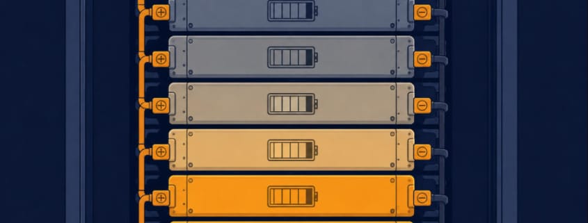
Mixed-Age String Design: Managing a BESS String After Augmentation Adds New Cells
Mixed-age string design is the problem every DC-shuffled augmentation eventually runs into. New modules and years-old modules end up sharing hardware.
The BMS then has to make that mix actually work. Our BESS augmentation guide and our AC block addition vs. DC shuffling comparison cover whether to augment and whether to add capacity on the AC or DC side.
This article picks up after that decision. Once new and old modules are physically on site together, mixed-age string design becomes the question that matters.
It’s narrower and more technical: how do you run a string that mixes cells at very different points in their degradation curve? And how do you do it without dragging new capacity down to old capacity’s level?
What is Mixed-Age String Design in BESS?
Mixed-age string design means managing a BESS string where old and new modules share hardware after augmentation. A series string’s weakest module caps its capacity, so mixing ages often pulls new capacity down. Segregating old and new modules into separate strings usually preserves more capacity than mixing them.
Key Takeaways for BESS Mixed-Age String Design
- Weakest-Link Capacity Cap: A series string’s total usable capacity is limited by its most degraded module, preventing newly added modules from delivering full rated power.
- Impedance & Degradation Mismatch: Resistance differences between old and new cells create uneven electrical and thermal stress, accelerating divergent degradation under load.
- Module Segregation Strategy: Grouping modules into separate strings by State of Health (SOH) preserves significantly more capacity than mixing old and new cells within a single string.
- Joint Constraint Sorting: Multi-variable assembly algorithms (matching capacity, impedance, and self-discharge) reduce cell mismatch by 76–87% compared to single-metric sorting.
- String-Level BMS Control: BMS and EMS logic must manage cutoffs and dispatch priorities at the string level rather than the whole-pack level to protect new capacity.
Why Mixed-Age String Design Is a Real Engineering Problem
Augmentation sounds simple on paper. Add new modules, restore lost capacity, move on.
The DC-shuffling path makes mixed-age string design harder than it sounds. New modules added this way often end up wired into the same series string as modules that have already lost real capacity.
Years of cycling and calendar aging cause that loss. However, it doesn’t happen evenly across a fleet.
In a series-connected string, the weakest module caps total usable capacity. The string can’t deliver more than its most degraded member allows before hitting a cutoff. Peer-reviewed research on active balancing for serially connected battery packs confirms this constraint directly: without balancing, the lowest-capacity cell in a series string limits the capacity the whole string can deliver.
A brand-new module wired into an old string doesn’t contribute its full rated capacity to the pack. It gets pulled down to whatever the weakest module in that same string can still deliver.
Mixed-age string design is the discipline of avoiding that outcome. It works through physical string assembly, BMS cutoff logic, or both.
The Weakest-Link Problem: How New Capacity Gets Dragged Down
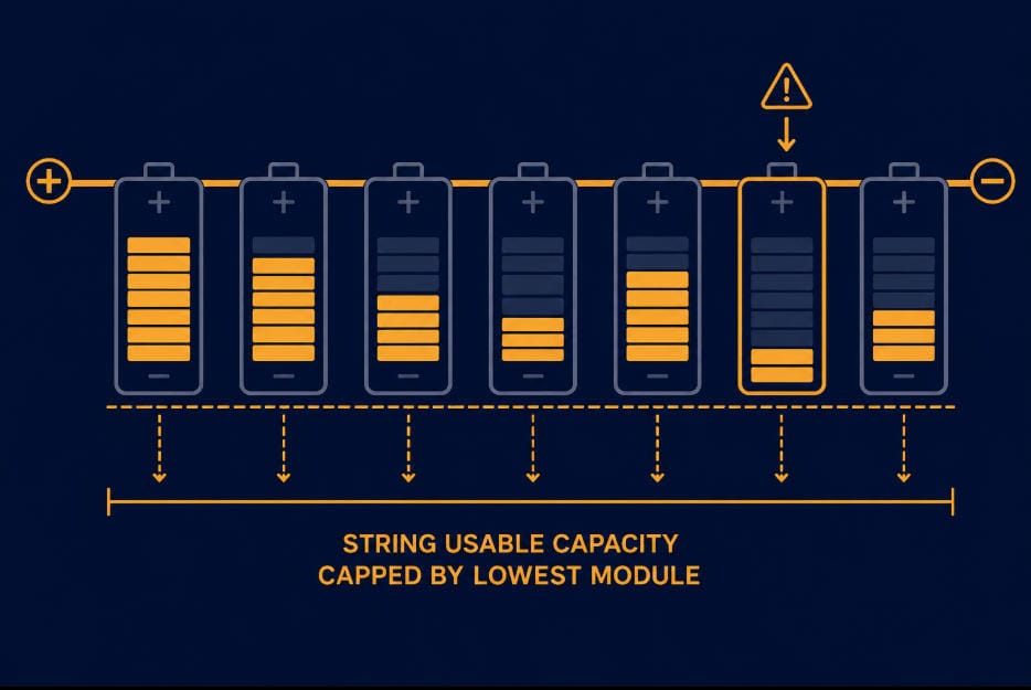
The mechanism is straightforward once you see it. Cells or modules in series all carry the same current. Voltage, not current, is what varies between them.
As the string discharges, the most degraded module reaches its low-voltage cutoff first. It has the least remaining capacity. The BMS has to stop the whole string there.
That happens regardless of how much charge the newer modules still have left. The same happens in reverse on charge.
The weakest module hits its upper voltage limit first. The whole string stops charging there too, even if the new modules could still accept more.
Impedance mismatch compounds the problem. A 2014 study on parallel-connected lithium-ion cells found that a 20% internal-resistance difference between two cells led to roughly a 40% reduction in cycle life.
While parallel sets suffer from uneven current sharing, this mechanism directly impacts series strings as well: higher-impedance modules in series generate greater localized heat under load, creating thermal hotspots that accelerate degradation across the entire string.
Separate experimental work on parallel-connected cells under thermal gradients found a related pattern: a 30°C thermal gradient across a pack roughly doubled the degradation rate and produced 50% more capacity loss after 1,000 cycles.
Both results are from parallel-connected cells specifically, not a series-string augmentation case. But the underlying mechanism generalizes.
Impedance mismatch between old and new modules creates uneven electrical and thermal stress. That stress tends to widen the gap between them, not close it.
BMS and EMS Strategies for Mixed-Age String Design
Matching Modules Before They Go Into a String
The first lever is physical: which modules actually get grouped into which string.
A 2026 optimization study on assembling heterogeneous battery packs from repurposed cell inventories tackled this directly. The study targeted second-life EV packs, not BESS augmentation, but used the same string-assembly logic.
It used a mixed-integer linear program to jointly minimize capacity spread, internal resistance spread, and self-discharge spread across a string, rather than sorting by one metric alone.
That joint approach cut mismatch by 76-87% compared to simple single-metric sorting — grouping modules by capacity alone, or resistance alone, and hoping the rest lines up.
The practical takeaway for mixed-age string design: sorting new and old modules by one number, like nameplate capacity, leaves real mismatch on the table. Impedance and self-discharge rate matter just as much.
Segregating Strings by Health Instead of Mixing Them
The second lever is architectural: don’t mix ages within one string at all.
Research on heterogeneous reconfigurable battery systems notes that prior SoH-aware reconfiguration studies show grouping cells of similar health within the same series string improves delivered pack capacity.
The logic holds because a string’s usable capacity is still constrained by its weakest member either way. Grouping by health just keeps that weakest member from dragging down modules that don’t belong with it.
Applied to mixed-age string design, this points toward keeping new modules in their own dedicated strings. Therefore, they should remain separate from the legacy fleet, wherever the site’s busbar and rack layout allow it.
Each string can then run its own SOH-appropriate cutoffs. The new string isn’t held back by the old one. The old string isn’t pushed harder trying to keep pace with modules it can no longer match.
Mixed-Age String Design: Setting Cutoffs and Dispatch at the String Level
Whichever physical layout a site ends up with, the BMS and EMS configuration has to follow it.
A single pack-wide cutoff voltage, sized for the newest modules, risks over-discharging or over-charging the old ones.
A cutoff sized for the oldest modules protects them. But it wastes real capacity sitting unused in the new modules every single cycle.
Per-string or per-block SOH tracking, feeding into a shared control layer, avoids that trade-off. It’s the same shared-state pattern covered in our integrated BMS control architecture guide — mixed-age string design is one more reason that architecture earns its complexity.
On the EMS side, operators can also set dispatch priority deliberately. Favoring the newer string during high-stress events — fast frequency response, high-C-rate calls — protects its cycle life.
Reserving the older string for gentler duty does the same in reverse, instead of averaging stress evenly across mismatched hardware.
Mixed-Age String Design: Segregated Strings vs. Mixed Strings
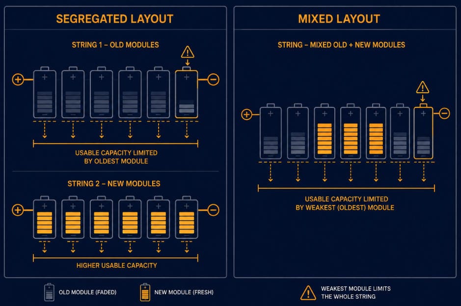
Neither approach is free. Segregation asks more of the site’s electrical layout; mixing asks more of the BMS.
| Factor | Segregated Strings (old and new separate) | Mixed Strings (old and new combined) |
| Delivered new-module capacity | Close to full rated capacity | Reduced — capped by the weakest module in the shared string |
| BMS/EMS complexity | Lower per string; needs per-string SOH tracking at the control layer | Higher — cutoffs must reconcile two very different degradation states in real time |
| Physical/electrical requirement | Needs spare busbar/breaker capacity for a genuinely separate string | Fits within existing string wiring, easier where space is tight |
| Best fit | Sites with layout headroom, or where preserving new capacity matters most | Sites with hard busbar/space constraints and modest capacity mismatch |
This decision sits downstream of the AC-vs-DC augmentation choice covered in our AC block addition vs. DC shuffling guide. AC block addition sidesteps mixed-age string design entirely, since the new block runs on its own inverters.
It never shares a string with the old fleet. DC shuffling is where this problem actually shows up.
Frequently Asked Questions
Does mixed-age string design apply to AC block addition too?
Not directly. AC block addition installs a new, self-contained power block with its own inverters. The new modules never share a DC string with the old fleet.
Mixed-age string design is specifically a DC-shuffling problem, since that path reuses the existing DC bus and wiring.
How much capacity is actually lost by mixing old and new modules in one string?
It depends on how degraded the old modules are relative to the new ones. A series string’s weakest module caps its usable capacity, so the loss scales with that gap.
A small gap between oldest and newest modules costs little. A large gap can waste a meaningful share of the new capacity added.
Can a BMS correct for mixed-age imbalance with active balancing alone?
Active balancing helps with cell-level SOC drift within a string. It doesn’t remove the underlying capacity or impedance gap between old and new modules.
Balancing hardware and string-level design address different parts of the same problem — see our active balancing topologies guide for how the hardware itself works.
Is segregating strings always the better choice?
Not always. It preserves more new capacity, but it needs spare busbar and breaker headroom the existing site layout may not have.
Where space is tight, a mixed string with carefully matched modules and string-appropriate cutoffs can still be the more practical choice.
Further Reading
BESS Augmentation: The Complete Guide to Restoring Capacity Lost to Degradation
BESS Augmentation: AC Block Addition vs. DC Shuffling
In-Service Cell Imbalance in LFP BESS
Integrated BMS Control Architecture
Active Balancing Hardware Topologies Compared
Sources
- Optimal Assembly of Repurposed Lithium-Ion Battery Packs under Cell Heterogeneity and Screening Uncertainty. arXiv:2607.12951 (2026)
- Target-Mean State-of-Charge Control for Maximum Utilization of Heterogeneous Reconfigurable Battery Systems Under Constant-Bus Constraints. Batteries 2026, 12, 221. MDPI (peer-reviewed, open access)
- Degradation in parallel-connected lithium-ion battery packs under thermal gradients. Communications Engineering (Nature), 2024
- Gogoana, R.; Pinson, M.B.; Bazant, M.Z.; Sarma, S.E. Internal resistance matching for parallel-connected lithium-ion cells and impacts on battery pack cycle life. Journal of Power Sources 252 (2014), 8-13
- A novel active cell balancing topology for serially connected Li-ion cells in the battery pack for electric vehicle applications. PMC (peer-reviewed, open access)