
How Temperature Accelerates Battery Degradation: The Arrhenius Relationship in LFP Cells
Every BESS guide tells you to keep cells cool. Fewer explain why temperature has such an outsized effect in the first place. The Arrhenius relationship between temperature and battery degradation answers that question. It is not a rule of thumb. Instead, it is real chemistry. Understanding it changes how you think about thermal design.
This guide skips the practical checklist most temperature guides repeat. It explains the actual mechanism instead. First, it covers what the Arrhenius equation says. Then it covers why that equation applies to batteries at all. Then it covers a detail most guides skip. Cold accelerates aging too, through a completely different pathway than heat. Finally, it covers what this means for BESS design at scale.
| Quick Answer The Arrhenius relationship between temperature and battery degradation describes how chemical reaction rates, including the ones that degrade a battery, scale exponentially with temperature. As a rough rule, degradation reactions roughly double in rate for every 10°C increase. This is not linear. A cell running 20°C hotter than another does not age twice as fast. It can age four times as fast or more. |
Temperature Battery Degradation Arrhenius: What the Equation Actually Says
Chemistry students learn the Arrhenius equation for a reason. It shows up almost everywhere reaction rates matter. Battery degradation is, at its core, a reaction rate problem.
The equation behind the Arrhenius relationship between temperature and battery degradation is simple in shape. It links reaction rate to temperature through one key number: activation energy. Every chemical reaction needs a minimum amount of energy to proceed. This includes the side reactions that consume lithium inside a cell. Temperature sets how many molecules have enough energy to clear that bar at any given moment. Raise the temperature, and more molecules clear it. The reaction speeds up. It speeds up exponentially, not in a straight line.
This is why a common shorthand holds up well across a useful range. Degradation roughly doubles for every 10°C rise. It is a simplification of the real curve. Still, it captures the core idea. Small temperature increases produce big jumps in degradation rate.
Why Activation Energy Varies by Material
First, not every part of a battery responds to temperature the same way. Activation energy is specific to each material and each reaction. That number determines how sensitive a given process is to heat.
Research measuring activation energy across battery materials found real differences. This number is a key input for modeling the Arrhenius relationship between temperature and battery degradation. Graphite, the typical anode material, showed a low activation energy of about 0.025 eV. LFP, by contrast, showed a notably higher activation energy of about 0.116 eV. A higher activation energy generally means a steeper response to temperature changes. That shows up in how the material conducts and how it ages. Worth noting: this figure comes from a battery-testing equipment vendor’s own case study, not a peer-reviewed paper. The methodology is transparent and the number checks out, but it sits in a different sourcing tier than a journal citation.
This matters for a simple reason when applying the Arrhenius relationship between temperature and battery degradation to a real system. Generic degradation guidance often gets built around chemistries like NMC, not LFP specifically. Borrowing that number for an LFP system can produce a genuinely wrong degradation estimate. Accurate modeling needs an activation energy number that matches the real chemistry in the cell.
Temperature Battery Degradation Arrhenius: Why Cold Also Accelerates Aging
Most practical guides frame temperature as a single dial. Hotter is worse, colder is better, full stop. But the real picture is more interesting than that. It matters for how you design a system.
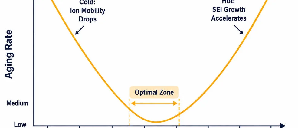
Research plotting battery aging rate against temperature found something specific. That research plotted the Arrhenius relationship between temperature and battery degradation directly. It is a V-shaped curve. Aging rate is not lowest at the coldest temperature tested. Instead, it hits a minimum at some optimal middle temperature. Then it rises again as conditions get colder still. Both ends of the curve show accelerated aging. Only the mechanism differs. Worth noting: the underlying study used NCA and NMC111 cells, not LFP. The V-shape itself is generally treated as chemistry-general in the literature, but the exact crossover point likely shifts somewhat for LFP specifically.
First, on the hot side, the story is the one covered above. Heat speeds up SEI growth and other side reactions directly. This runs through the same Arrhenius relationship covered above. For the deeper chemistry behind that specific mechanism, see our guide on SEI Layer Growth and Lithium Plating in LFP Cells. It covers the heat-driven side in full.
Then on the cold side, the mechanism is different. First, ion mobility slows down. Then internal resistance rises. Under high current in the cold, this can push cells toward lithium plating conditions. That is a different, worse outcome than simple slow aging. Instead, the V-shape is not really one curve. Instead, it is two separate degradation pathways overlapping. One dominates at high temperature. The other dominates at low temperature. A sweet spot sits in between, where both are minimized.
Temperature Battery Degradation Arrhenius and the Calendar vs Cycle Aging Link
Temperature does not degrade a battery through one single pathway. Instead, it touches both of the two aging processes that run in every cell at once.
Calendar aging is the slow degradation that happens even at rest. It follows the Arrhenius relationship closely. A cell sitting idle in a hot enclosure loses capacity faster than an identical cell sitting idle in a cool one. That difference comes purely from elevated reaction rates. Cycle aging is the degradation from active charging and discharging. It gets a second temperature effect layered on top. Heat during active cycling adds mechanical and chemical stress. This goes beyond what calendar aging alone would predict.
For the full breakdown of how these two aging pathways interact, see our guide on Calendar Aging vs Cycle Aging in LFP Batteries. It covers how operators separate them in real data. Temperature is the variable that connects both halves of that picture.
Applying This at BESS Scale: Why Uniformity Matters as Much as Average Temperature
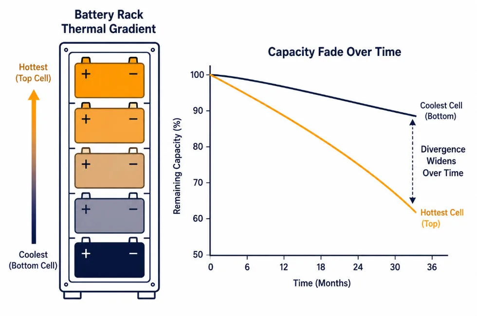
Individual cell chemistry is only half the story. A BESS is not one cell. Instead, it is thousands of cells. The Arrhenius relationship has a brutal implication for how they age together.
Degradation rate scales exponentially with temperature, not in a straight line. Small temperature differences between cells in the same rack do not average out. Instead, they compound. A cell running just a few degrees hotter than its neighbors ages meaningfully faster on its own. This can come from airflow patterns or its position in the rack. Over years of operation, that early divergence widens rather than closing. The hotter cell keeps aging faster at every step.
This is exactly why temperature uniformity across a BESS matters as much as the average temperature target. For the detailed engineering breakdown of safe temperature spread limits, see our guide on Cell Temperature Gradients in BESS. It covers what causes uneven heating in a rack. The Arrhenius relationship explained here is the underlying reason that guide’s ΔT limits exist in the first place.
Putting a Number on It: A Simple Arrhenius Comparison
The exponential relationship is easier to trust with a concrete example. Take two identical LFP cells. One runs at a steady 25°C. The other runs at 45°C, a 20°C difference that is common between a well-cooled and a poorly-cooled enclosure.
Using the 10°C-doubling shorthand, the hotter cell does not age 20% faster or even 50% faster. It ages roughly four times faster, since two separate 10°C jumps each roughly double the rate. A design choice that looks like a modest thermal compromise on paper can matter a lot in practice. It can translate into a dramatically shorter real-world service life. This is the practical payoff of understanding the Arrhenius relationship instead of just following a cooling checklist blindly.
The same logic applies in reverse. Pulling a system from 45°C down to 35°C can meaningfully extend service life. That is still a fairly warm operating point. It still runs warmer than the 25°C reference point most datasheets use. Incremental cooling improvements pay off at every point along the curve, not just at the extremes.
What This Means for Thermal Design Choices
None of this changes the practical playbook much. Still, it explains why that playbook works the way it does.
Liquid cooling outperforms air cooling on more than comfort. It holds cells within a tighter temperature band. It also reduces cell-to-cell spread. Both matter directly because of the exponential relationship covered above. For the full comparison of cooling approaches, see our guide on Liquid vs Air Cooling System Use in BESS. It covers the tradeoffs in detail. Cold-climate design deserves the same weight as hot-climate design, not less. The V-shaped curve means both extremes carry real degradation risk. For that side of the picture, see our guide on Cold-Climate BESS Design. It covers discharge-side cutoffs in cold weather.
For a practical, rule-of-thumb breakdown of temperature’s effect on cycle life, see our existing guide on Impact of Temperature on LiFePO₄ Batteries Cycle Life. It applies the 10°C-doubling shorthand to real cycle numbers. That guide covers the practical numbers. This one covers the mechanism behind them.
Temperature Battery Degradation Arrhenius: Quick Reference
| Factor | What It Means |
| Core relationship | Degradation rate scales exponentially with temperature, not linearly |
| Common shorthand | Roughly doubles per 10°C temperature increase |
| Activation energy | Chemistry-specific; higher values mean steeper temperature sensitivity |
| Hot-side mechanism | Accelerated SEI growth and side reactions |
| Cold-side mechanism | Slower ion mobility, higher resistance, elevated plating risk under load |
| Curve shape | V-shaped, with a minimum-aging point, not a straight line |
| BESS-scale implication | Uniformity matters as much as average temperature, due to compounding |
Frequently Asked Questions
In the Arrhenius relationship between temperature and battery degradation, does the 10°C-doubling rule apply exactly, or is it a simplification?
It is a simplification. The real relationship is a smooth exponential curve. The doubling shorthand holds up reasonably well across a normal operating range. Still, it is an approximation, not an exact law.
Why does LFP have a different activation energy than other chemistries?
Activation energy depends on the specific materials and reactions involved. LFP’s cathode chemistry behaves differently from NMC or NCA under the same conditions. Its measured activation energy differs as a result. Generic lithium-ion guidance does not always transfer cleanly as a result.
Is cold temperature ever actually good for battery life?
There is a minimum-aging point, and it sits below room temperature for some cells. But going too cold introduces its own accelerated aging pathway. Slower ion mobility and higher plating risk drive it. Colder is not simply better without limit.
Under the Arrhenius relationship between temperature and battery degradation, does uniformity really matter more than average temperature?
Both matter, but uniformity is the more commonly underestimated factor. Degradation compounds exponentially. A hotter pocket of cells in an otherwise well-managed system can become a persistent weak point. Over time, that weak point drags down pack-level performance.
Further Reading
Battery Degradation in BESS: Causes, Mechanisms & Mitigation
SEI Layer Growth and Lithium Plating in LFP Cells
Calendar Aging vs Cycle Aging in LFP Batteries
Impact of Temperature on LiFePO₄ Batteries Cycle Life
Cold-Climate BESS Design: Discharge-Side DCIR and Premature Cutoffs
SEI Layer Growth and Lithium Plating in LFP Cells
Every LFP cell carries two chemistry problems that quietly shape its whole life. Together, these two problems make up SEI layer growth and lithium plating, the pairing this whole guide covers. First, one is slow and mostly unavoidable. Then the other is fast and mostly preventable. So understanding how each one works is the difference between managing degradation and just watching it happen.
So this guide explains both mechanisms from the ground up. First, it covers what the SEI layer actually is and why it keeps growing. Then it covers how lithium plating happens, and why it is so much more damaging. Along the way, it links to the operating guidance that follows from the chemistry.
| Quick Answer SEI layer growth is the slow, ongoing thickening of a protective film on the anode, driven mainly by time and high state of charge. Lithium plating is the sudden deposit of metallic lithium on the anode surface, triggered by fast charging in cold conditions. SEI growth is a normal aging process. Lithium plating is largely avoidable damage. |
SEI Layer Growth: What the Film Actually Is
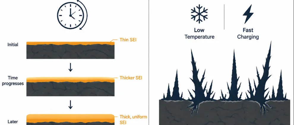
Every lithium-ion cell forms a thin film on the anode surface early in its life. Understanding SEI layer growth and lithium plating starts here, with this first film. That film is the solid electrolyte interphase, or SEI. It is not a flaw. Instead, it is a necessary part of how the cell works at all.
The SEI forms when electrolyte comes into contact with the anode and partially decomposes. That reaction consumes a small amount of lithium and electrolyte. But in exchange, it builds a protective layer. This layer lets lithium ions pass through while blocking further direct contact between the anode and electrolyte. Without it, the electrolyte would keep breaking down uncontrollably.
So a stable SEI is good news, up to a point. It settles into a thin, mostly fixed layer during the cell’s first few cycles. That initial formation consumes some capacity, which is normal and expected. Manufacturers account for it before the cell ever reaches a customer.
SEI Layer Growth: Why It Keeps Going After That
Here is the problem. But the SEI does not stay fixed forever. Instead, it keeps growing, slowly, for the entire life of the cell. Each time it thickens, it consumes a little more lithium and electrolyte. That lithium never comes back.
Two conditions speed this up. State of charge is the biggest one. Then temperature is close behind. A cell held at high state of charge sees faster SEI growth than one kept in a mid-range window. This is especially true near 100%. Heat accelerates the same underlying chemical reactions too. A hot cell ages faster than a cool one, even at the same state of charge.
This slow growth is exactly what shows up as calendar aging at the system level. It is the quiet, background half of SEI layer growth and lithium plating. For the full picture on how SEI growth connects to calendar and cycle aging together, see our guide on Calendar Aging vs Cycle Aging in LFP Batteries. It covers the aging side of SEI layer growth and lithium plating in more depth.
The growing SEI layer also raises internal resistance. Instead, lithium ions have to pass through a thicker barrier to reach the anode. That barrier resists ion flow more with every passing month. This is why aging cells run measurably hotter and less efficiently than new ones. This shows up even before capacity loss becomes obvious.
Lithium Plating: What It Actually Is
Lithium plating is a different problem entirely, and a more dangerous one. Of the two halves of SEI layer growth and lithium plating, this is the fast, event-driven one. Instead of lithium ions intercalating cleanly into the anode’s graphite structure, they deposit on the surface as metallic lithium. That metallic lithium does not behave like the lithium safely stored inside the graphite. Much of it becomes permanently unusable.
The trigger is specific. Lithium plating happens when the anode cannot absorb lithium ions fast enough to keep up with the charging current. Researchers have shown this occurs once the graphite electrode’s potential drops to roughly zero volts versus lithium metal. Below that point, the physics favors plating over intercalation.
Two conditions push a cell toward that threshold. First, fast charging is one. Then cold temperature is the other, and the two compound each other badly. Cold slows lithium-ion mobility inside the electrolyte and the anode. The same charge current that is safe at room temperature can trigger plating in the cold. This risk kicks in once the cell drops below roughly 0°C. That is why charging below freezing gets treated as a hard BMS cutoff on LFP systems. It is not just a soft warning.
SEI Layer Growth vs Lithium Plating: Why One Is So Much Worse
SEI growth is slow and largely unavoidable. But lithium plating is different on both counts. This contrast is the core of why SEI layer growth and lithium plating get treated so differently in BMS design.
First, plated lithium is mostly unrecoverable. Once metallic lithium deposits on the anode surface, only a portion of it can re-intercalate on the next discharge. The rest becomes what researchers call dead lithium, permanently disconnected from the working electrochemistry. Every plating event removes real capacity that never returns.
Second, plating creates a safety risk that SEI growth does not. Repeated plating can build up as dendrites, needle-like structures that grow with each cycle. In the worst case, a dendrite can pierce the separator between the anode and cathode. That can cause an internal short circuit. This is why lithium plating gets treated as a hard safety limit in BMS design. It is not just a performance concern.
Third, plated lithium accelerates SEI growth on top of everything else. Fresh metallic lithium is highly reactive with the electrolyte. It forms its own new SEI layer directly on the plated lithium. That consumes even more lithium and electrolyte than normal SEI growth alone would. One plating event can trigger a small cascade of additional degradation beyond the initial capacity loss.
How SEI Layer Growth and Lithium Plating Interact
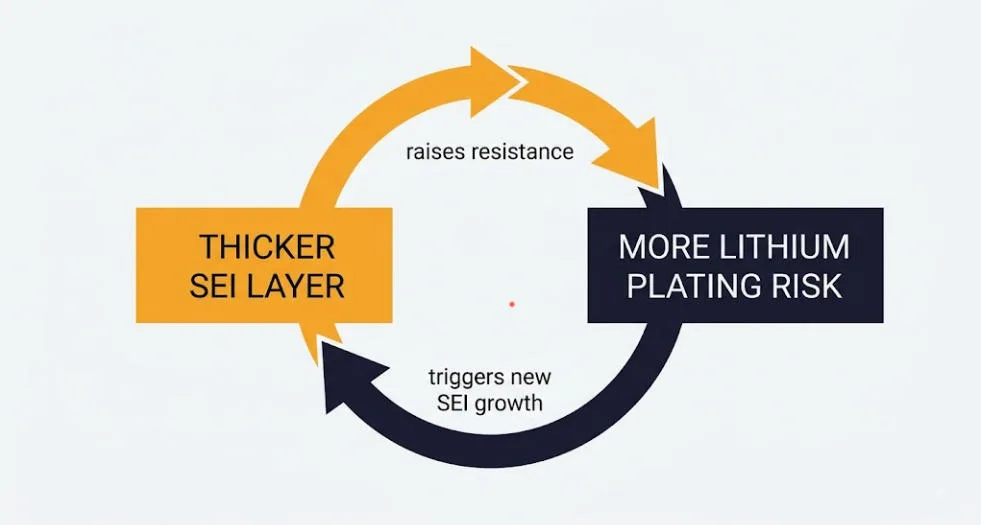
SEI layer growth and lithium plating are not fully separate stories. Instead, they feed into each other in both directions.
A thick, resistive SEI layer makes plating more likely at a given charge rate. As the SEI grows over a cell’s life, it adds resistance the charging current has to overcome. An older cell with a thicker SEI can start plating sooner. Charge rates and temperatures that were once safe stop being safe. This is one reason charge current limits often get more conservative as a system ages. It is not just a fixed spec on day one.
In the other direction, any lithium plating event accelerates SEI growth, as covered above. A single cold-weather charging mistake does not just cost the plated capacity directly. It also leaves behind a thicker SEI layer that keeps consuming a little more capacity on every cycle afterward.
This two-way relationship is part of why temperature management matters so much for LFP systems overall. It is the practical payoff of understanding SEI layer growth and lithium plating together, not as two unrelated topics. For the operational side of managing SEI layer growth and lithium plating, including BMS charge cutoffs and derating strategies, see our guides on Charging Temperature and Battery Datasheets and BESS C-Rate Explained. Still, both cover how real systems protect against plating in the field.
SEI Layer Growth and Lithium Plating: Detecting Damage Before It Spreads
Lithium plating does not always announce itself obviously in real time. That makes prevention more important than detection. Still, a few signals can flag it after the fact.
A sudden, disproportionate capacity drop following a cold-weather fast charge is one warning sign. So is a voltage plateau or dip during the charge itself. Either one can signal the anode potential crossing into plating territory. Post-mortem analysis using incremental capacity analysis can also reveal plating-related changes in a cell’s charge curve. These changes look distinct from the gradual shifts caused by ordinary SEI growth and cycle aging.
For the full detail on incremental capacity analysis and other degradation-tracking methods, see our guide on Advanced SOH Estimation for BESS. It covers how operators track these effects in a live system.
SEI Layer Growth and Lithium Plating: Practical Takeaways for BESS Operators
None of this SEI layer growth and lithium plating chemistry requires a battery science degree to manage well. A few operating habits cover most of the risk.
Keep resting state of charge out of the high extreme when possible, since that slows SEI growth directly. Respect temperature-based charge cutoffs strictly, especially near freezing, since that is the single biggest lever against plating. Avoid unnecessarily aggressive fast charging in cold weather, even when a system technically allows it. Allowed and optimal are not the same thing. Also, expect charge limits to tighten somewhat as a system ages. A thicker SEI layer genuinely does lower the safe charging threshold over time.
For the bigger picture on how SEI layer growth and lithium plating fit into overall battery degradation, see our guide on Battery Degradation in BESS: Causes, Mechanisms & Mitigation.
SEI Growth vs Lithium Plating: Quick Comparison
| Factor | SEI Layer Growth | Lithium Plating |
| Speed | Slow, continuous | Fast, event-driven |
| Trigger | Time and high state of charge | Fast charging in cold temperatures |
| Avoidable? | Mostly not, but can be slowed | Largely, with correct charge limits |
| Reversibility | Permanent but gradual | Largely permanent, some immediate loss |
| Safety risk | Low | Higher, dendrite/short-circuit risk |
| Main mitigation | Avoid high resting SOC, manage heat | Respect cold-temperature charge cutoffs |
Frequently Asked Questions
Does SEI layer growth ever stop?
No. It continues for the entire life of the cell, though the rate slows somewhat after the initial formation period. It never fully stops.
Can lithium plating be reversed?
Mostly no. A portion of plated lithium can re-intercalate on the next discharge. But the rest becomes permanently disconnected dead lithium. Prevention is far more effective than any recovery after the fact.
Why is lithium plating worse in cold weather specifically?
Cold temperatures slow lithium-ion mobility. This happens in both the electrolyte and the anode. That makes it harder for ions to intercalate quickly. The anode potential gets pushed toward the threshold where plating occurs instead.
Does a thicker SEI layer make lithium plating more likely?
Yes. A thicker, more resistive SEI layer adds to the overpotential during charging. That can push an aging cell toward plating conditions at charge rates that were once safe.
Further Reading
Battery Degradation in BESS: Causes, Mechanisms & Mitigation
Calendar Aging vs Cycle Aging in LFP Batteries
Advanced SOH Estimation for BESS
Charging Temperature: Why Battery Datasheets Often Miss Critical Charge Limits
Advanced SOH Estimation for BESS: Kalman Filtering and Machine Learning Methods
Every BESS needs a trustworthy answer to one question. How much capacity is left? That answer is state of health, or SOH. So what advanced SOH estimation BESS platforms rely on goes well beyond those basics. Instead, it moves past simple counting into methods that update continuously and catch what simpler tools miss.
Still, the basics matter too. Capacity counting, incremental capacity analysis, and resistance tracking cover the fundamentals well elsewhere. So this guide picks up where those leave off. Instead, it focuses on the model-based and data-driven methods that power modern, production-grade BMS platforms.
| Quick Answer Advanced SOH estimation for a BESS relies mainly on two approaches. Model-based methods, led by the Extended Kalman Filter, combine a battery model with real-time data to estimate SOH continuously. Data-driven methods train on historical data to predict SOH directly from patterns. Most production systems layer these with basic methods rather than using either alone. |
Why Basic Methods Fall Short: The Case for Advanced SOH Estimation BESS Tools
Capacity counting is accurate. But it takes the asset offline for hours. Incremental capacity analysis needs slow, steady charge rates. A hard-cycling BESS rarely gets those conditions. Resistance tracking is fast. But it does not always move in step with capacity fade.
So each basic method has a real gap that advanced SOH estimation BESS tools are built to fill. First, it runs continuously. Then, it does not need a dedicated test cycle. Also, it can fuse multiple weak signals into one stronger estimate.
For the full detail on capacity counting, incremental capacity analysis, and resistance-based tracking, see our guide on BMS Algorithms Explained. It covers those foundational methods in depth. Our guide on DCIR and BESS Performance covers resistance-based tracking specifically. So the rest of this guide builds on that foundation.
Advanced SOH Estimation BESS Method: Kalman Filtering
How the Extended Kalman Filter Works
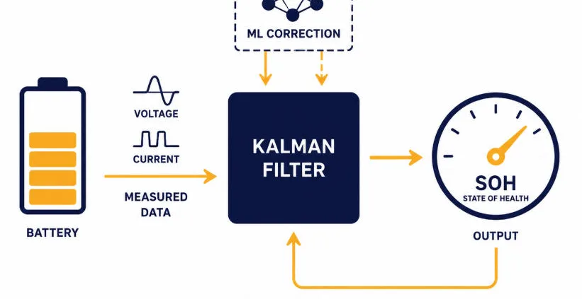
Model-based methods take a different approach entirely. Instead of measuring capacity directly, they combine a mathematical battery model with real-time voltage and current data. Then SOH comes out as one of several hidden values inside that model.
The Extended Kalman Filter, or EKF, is the most common tool here. So it treats SOH as a state that evolves slowly over time. Then SOC, by contrast, is a state that evolves quickly. So both get updated together as new voltage and current readings arrive. This is the core mechanism behind what advanced SOH estimation BESS platforms rely on for continuous tracking. No dedicated test cycle is needed at all.
So this is where advanced SOH estimation BESS platforms really separate from basic tracking altogether. Instead, an EKF does not wait for a full cycle or a clean charge curve. So it updates with every new data point, all day, every day. So that is a fundamentally different operating mode than periodic testing.
Still, the catch is model dependency. An EKF is only as good as the battery model feeding it. A model that misses LFP’s flat voltage curve and hysteresis will shake. Its SOH estimate will wobble too. This is the same modeling challenge that shows up in SOC estimation too. See our guide on BMS SOC Estimation Methods Explained for the deeper dive. The underlying model quality issue is shared between SOC and SOH filtering.
Kalman Filter Variants Worth Knowing
Beyond the standard EKF, several variants push accuracy further still. First, the Unscented Kalman Filter handles the battery’s nonlinear behavior more directly, at higher computational cost. Dual and joint Kalman filters estimate SOC and SOH together, side by side. Each one helps the other. They do not run as separate, disconnected calculations. Adaptive Kalman filters go further still. They adjust their own noise settings as the battery ages. So the filter does not quietly get worse as the cell drifts from its original model.
So research comparing filter types generally finds Kalman-based approaches outperform simple coulomb counting or raw voltage lookups on accuracy. But that accuracy gain depends entirely on getting the underlying model right first. A poorly tuned EKF can do worse than a well-calibrated simple method. That is why checking the model matters as much as picking the filter.
Advanced SOH Estimation BESS Method: Data-Driven and Machine Learning
How Data-Driven SOH Estimation Works
The newest category skips chemistry modeling almost entirely. So this data-driven approach is a growing part of advanced SOH estimation that BESS platforms increasingly adopt as fleets scale up. Instead, a data-driven system trains on historical voltage, current, resistance, and temperature data. It learns to predict SOH straight from patterns in that data. No engineer needs to hand-build the physics behind it.
Still, these methods can be very accurate once trained on enough data from similar cells. Some published results report SOH prediction errors under 1%. But they carry a real cost. So training requires a large, representative dataset covering realistic aging conditions. A model trained on one usage pattern may not work on a very different one. So data-driven methods work well for fleet-scale operators with lots of historical data. They work less well for a single small system starting from scratch.
Common Model Types
So a few model types show up again and again in this space. Neural networks handle battery data well, since it comes in sequence. Recurrent architectures like LSTMs work especially well here, since today’s SOH depends heavily on yesterday’s usage pattern. Then gradient-boosted tree models offer a lighter option. They need less training data, at some cost to peak accuracy. Gaussian process regression adds something useful. It gives a confidence range around each prediction. That matters for operators who need more than just a number. They need to know how much to trust it.
So hybrid approaches are increasingly common as a middle ground here too. A model might combine a physics-based EKF core with a machine learning correction layer. Then that layer is trained to catch what the physics model misses. So this blends two strengths. It keeps the clarity of model-based methods, and it gains some of the accuracy of data-driven ones. So for many fleet operators, this hybrid path offers the best of both without committing fully to either extreme.
How Advanced SOH Estimation Layers with the Basics in a Real BMS
So no single advanced SOH estimation BESS method covers every need on its own. Real BMS platforms typically layer several of these together, basic and advanced alike.
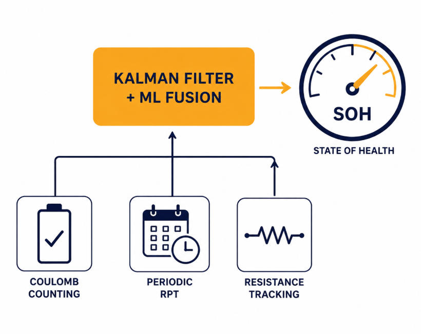
Coulomb counting runs continuously in the background. It is cheap, and it is always available. Periodic Reference Performance Tests reset the drift that coulomb counting accumulates over time. Resistance tracking via pulse tests adds a second, faster signal between full tests. Then a Kalman filter or similar model-based layer fuses all of that input together. Often, a machine learning correction sits on top. The result is one continuously updated SOH number the operator can actually act on.
This is the real payoff of advanced SOH estimation that BESS teams invest in. First, it is not about replacing the basics. Instead, it is about fusing them into something more reliable than any single input alone. The Kalman filter or ML layer acts as the integration point. It weighs each incoming signal by how much it should be trusted at that moment.
This layered approach connects directly to the Equivalent Full Cycle concept. That concept is used to separate calendar and cycle aging in field data. Both concepts feed the same underlying goal. That goal is a trustworthy, continuously updated picture of how much life a BESS has left. For more on how EFC-based tracking fits into the bigger degradation picture, see our guide on Calendar Aging vs Cycle Aging in LFP Batteries. It covers the full framework.
Reporting and Version Drift in Advanced SOH Systems
Still, however sophisticated the method, reporting matters as much as the calculation itself. A single SOH number without context can mislead. Is it a raw Kalman filter output, an ML prediction, or a blend of both? Was it measured fresh off a full Reference Performance Test, or purely interpolated by a model between tests? Advanced SOH estimation BESS dashboards that surface this context help operators trust the number instead of just reading it.
So version drift is a real risk for advanced SOH estimation BESS platforms running model-based and ML systems specifically. If a BMS updates its underlying model, the SOH number can jump. This holds true even when the battery itself has not changed. So it helps to log which method and model version produced each SOH reading, not just the number alone. That log becomes valuable later. It matters most when comparing degradation trends across a fleet of systems built at different times.
Choosing the Right Advanced SOH Estimation BESS Approach
The right level of advanced SOH estimation that BESS operators actually need depends on two things. System size is one. How the asset gets used is the other. A small residential or commercial system may get by fine with basic coulomb counting. Occasional full-capacity tests can fill the gap. Model-based methods can wait.
A large utility-scale asset generating revenue around the clock is a different story. It needs more from advanced SOH estimation BESS platforms. There, the added complexity of a full Kalman-filter or hybrid ML approach usually pays off. Even small SOH estimation errors translate into real dispatch and warranty costs at that scale. Fleet operators with many similar systems get the most value from data-driven methods. They have the training data those methods need to perform well.
Whatever the advanced SOH estimation BESS approach is chosen, the underlying goal stays the same. Accurate SOH tracking is what turns raw degradation into something an operator can actually plan around. For the broader mechanisms behind that degradation, see our guide on Battery Degradation in BESS: Causes, Mechanisms & Mitigation. It lays out the full picture.
Advanced SOH Estimation Methods: Quick Comparison
| Method | Speed | Accuracy | Best Fit |
| Kalman filter (EKF/UKF) | Continuous | High, if model is accurate | Real-time production systems |
| Dual/adaptive Kalman filter | Continuous | Higher, self-corrects over time | Long-life assets with aging models |
| Neural network / LSTM | Continuous | High, with enough training data | Fleet-scale operators with data |
| Gaussian process regression | Continuous | High, with confidence intervals | Operators needing uncertainty estimates |
| Hybrid physics + ML | Continuous | Highest, blends both strengths | Large fleets wanting best-in-class accuracy |
Frequently Asked Questions
What is the most accurate advanced SOH estimation BESS method available?
No single method wins universally. Hybrid approaches often report the best accuracy. They combine a physics-based Kalman filter with a machine learning correction layer. That combination captures known battery physics and the patterns pure physics models miss.
Do I need machine learning for SOH estimation, or is a Kalman filter enough?
For most single-site systems, a well-tuned Kalman filter is enough. Machine learning methods earn their added complexity mainly at fleet scale. That is where enough historical data exists to train a model well.
Why does a Kalman filter sometimes perform worse than simple coulomb counting?
So this happens when the underlying battery model is poorly calibrated. An EKF is only as good as the model feeding it. So a mismatched model can produce worse results than a simple, well-calibrated basic method.
Does advanced SOH estimation replace basic methods like coulomb counting in a BESS?
No. Advanced methods almost always layer on top of basic ones instead of replacing them. They fuse coulomb counting, periodic tests, and resistance signals into one stronger estimate.
Further Reading
Battery Degradation in BESS: Causes, Mechanisms & Mitigation
Calendar Aging vs Cycle Aging in LFP Batteries
BMS SOC Estimation Methods Explained: OCV vs Coulomb Counting vs Kalman Filter
BMS Algorithms Explained: SOH Estimation, SoP, SoE, Cell Balancing, and Safety Diagnostics
The Power Test: Why DCIR Is the True Measure of BESS Performance
Calendar Aging vs Cycle Aging in LFP Batteries
Every LFP battery in a BESS ages through two processes at once. One happens with the clock. The other happens with use. So calendar aging vs cycle aging is not really an either/or question. Also, both run all the time, and their effects stack together. Still, telling them apart matters. Still, each one responds to a different set of operating choices.
So this guide breaks calendar aging vs cycle aging down piece by piece, mechanism by mechanism. First, it covers what each process is on its own. Then it covers how the two interact in a real system. Finally, it covers how BESS operators separate the two in field data, since that is where the theory becomes useful.
| Quick Answer Calendar aging is time-based capacity loss that happens even when a battery is idle, driven mainly by state of charge and temperature. Cycle aging is use-based capacity loss driven by charge and discharge throughput, depth of discharge, and C-rate. Both processes run at once in a working BESS, and total degradation is roughly the sum of the two. |
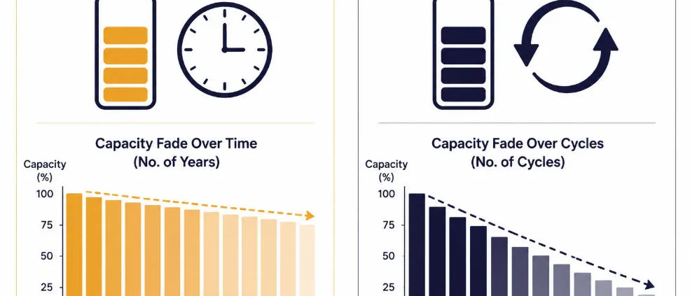
Calendar Aging vs Cycle Aging: What Calendar Aging Is
Calendar aging is capacity loss that happens purely with time. So it keeps going whether the battery is cycling, sitting idle, or somewhere in between. Think of it as a background process running underneath everything else.
The root mechanism is growth of the solid electrolyte interphase, or SEI layer, on the anode. So this layer forms naturally, and it even serves a protective role at first. But it keeps growing slowly for the life of the cell. Then each time it thickens, it consumes lithium and electrolyte. That lithium never comes back.
So two variables drive how fast this happens. State of charge is the biggest one. Then temperature is close behind. A cell parked at high state of charge ages faster at rest than one held in a mid-range window. This is especially true near 100%. So does a cell sitting in a hot enclosure compared to a cool one.
So research backs this up clearly. A 2025 study on LFP pouch cells backs this up. It found that calendar aging is strongly governed by state of charge and temperature together. So higher values of either sped up capacity fade through faster SEI growth. Pressure, by contrast, had almost no measurable effect. Interestingly, the same study found something less obvious. Still, cells stored at 50% state of charge showed the largest rise in direct current resistance. This held true once they reached a given state of health, even though their capacity fade was not always the fastest. So that is a reminder that calendar aging vs cycle aging does not always degrade capacity and resistance in lockstep.
Calendar Aging vs Cycle Aging: What Cycle Aging Is
Cycle aging is capacity loss caused by the act of charging and discharging. Instead, it scales with how much energy passes through the cell, not just how much time goes by. A battery cycled hard sees more stress per day than one cycled gently. This holds even if both sit at the same average state of charge.
So several variables drive cycle aging. Depth of discharge is one. C-rate is another. Also, the state-of-charge range used during cycling matters too. A cell cycled between 20% and 80% takes less stress than one cycled between 0% and 100%. This holds even across the same number of cycles. Then temperature during active cycling also plays a role, on top of its calendar-aging effect at rest.
A long-running study on a commercial LFP and graphite cell ran cycle aging tests for 885 days. So it used 19 separate test points. Then these covered different combinations of temperature, C-rate, depth of discharge, and state-of-charge range. The results let researchers build a model that predicts cycle-driven fade from those four inputs. That kind of multi-variable model shows why cycle aging is harder to summarize in one sentence than calendar aging. So calendar aging vs cycle aging simply depends on more moving parts on the cycle side.
Cycle aging also tends to show up differently than calendar aging on a capacity curve. First, early cycles often cause a fast initial dip. Then fade slows into a steadier, more linear decline for a long stretch. Then late in life, fade can speed up again as the cell approaches end of life. Calendar aging, by contrast, tends to follow a smoother square-root-of-time pattern from the start.
How the Two Interact
Calendar aging vs cycle aging is a useful framing. But the two are not fully independent in practice. So a battery’s operating history shapes both at once. Take state of charge between cycles as an example. So it is itself set by how the cell was last used. That link between the two processes is one reason pure separation only works cleanly in a controlled lab setting.
Still, most aging models treat calendar and cycle aging as additive. Total degradation is modeled as roughly the calendar-aging contribution plus the cycle-aging contribution, calculated separately and then combined. So this additive approach is not perfectly accurate at the edges. But it holds up well enough to be the standard in both research and commercial degradation models.
One nuance is worth knowing here. But temperature drives both processes, and not always to the same degree. Research on large-format LFP cells built for stationary storage backs this up. So it found that temperature has the dominant effect on total aging. Still, the specific cycling protocol played a smaller secondary role. So keeping a system cool helps both pathways at once, even though the mechanisms underneath are different. For more on how temperature interacts with degradation broadly, see our guide on Battery Degradation in BESS: Causes, Mechanisms & Mitigation. It covers the full picture beyond calendar aging vs cycle aging alone.
Separating the Two in Real Field Data
In a lab, calendar aging and cycle aging can be isolated cleanly. So researchers run two sets of cells. One set only sits idle. The other only cycles. But in a live BESS, that kind of separation is not possible. So every cell has some combination of both happening constantly.
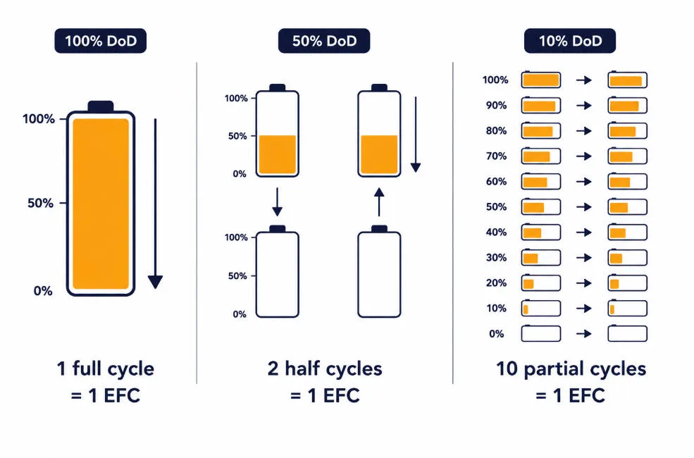
Operators handle this with a concept called the Equivalent Full Cycle, or EFC. An EFC converts partial cycles into a common unit based on energy throughput rather than raw cycle counts. So two 50% cycles count as one EFC. Ten 10% cycles also count as one EFC. So this puts shallow, frequent cycling and deep, occasional cycling on the same scale. That makes cycle-aging comparisons meaningful across very different usage patterns.
So with EFC as the throughput measure, operators can build a degradation model. It assigns a cycle-aging contribution per EFC and a calendar-aging contribution per unit of time. Then it sums the two. So LFP cells commonly rate between 2,500 and 9,000 EFC before reaching end-of-life thresholds. The exact number depends on the operating conditions and the EFC definition used. So that is a wide range. Still, cycling conditions like depth of discharge and C-rate largely explain why.
This EFC-based approach connects directly to how you track SOH in the field. Reference Performance Tests, run at fixed intervals, measure capacity and resistance directly. Between those tests, the EFC count and elapsed time both keep accumulating, feeding the additive model described above. For the full picture on tracking degradation as it happens, see our guide on BMS SOC Estimation Methods Explained. It covers how a BMS keeps that tracking accurate over time.
Modeling Calendar Aging vs Cycle Aging Together in a BESS
Most commercial degradation models treat calendar aging vs cycle aging as two curves added on top of each other. First, the calendar curve grows with elapsed time. Then the cycle curve grows with EFC count. At any point in a system’s life, total fade is close to the sum of both curves evaluated up to that point.
So this additive approach has a practical upside. It lets an operator run “what-if” scenarios without re-testing cells from scratch. Want to know how a change in dispatch strategy affects lifetime? Then increase the modeled EFC rate and hold the calendar term fixed. Want to know how a warmer siting location affects lifetime? Then adjust the temperature input feeding both curves and see how each one shifts.
Manufacturer degradation tables often build in this same logic, even when they present it as a single lookup chart. A table showing SOH by year and by cycling intensity is really just calendar aging vs cycle aging pre-combined into one surface. Reading the fine print on how that table was built tells you which usage pattern it assumes, which matters if your actual dispatch looks different.
Why the Distinction Matters for BESS Operators
Calendar aging vs cycle aging is not just an academic distinction. So calendar aging vs cycle aging changes what levers an operator actually has.
If calendar aging dominates a system’s degradation, the fix is mostly about resting state of charge and temperature. Idle capacity sitting at 100% SOC in a hot enclosure loses capacity every day, cycling or not. So that loss happens whether the asset is dispatched or parked. If cycle aging dominates instead, the fix is about how the system gets used. First, reducing depth of discharge helps. Then lowering C-rate helps too. Also, narrowing the SOC operating window targets cycle aging directly.
So most real systems have both pathways contributing. So the practical answer is usually “do both.” Keep resting SOC out of the high extreme when possible. Keep cells cool. Avoid unnecessary deep discharges. So none of these choices is exotic. What changes is which one matters most for a given system’s usage pattern. That depends on whether the system spends more of its life idle or more of its life cycling hard.
So application type is often the clearest signal. Take a solar-paired storage system as an example. It charges once a day, discharges once a day, and then sits mostly idle overnight. That pattern leans toward calendar-aging-dominant behavior. A frequency-regulation asset that cycles shallow and constant, day and night, leans toward cycle-aging-dominant behavior instead. So knowing which profile a system fits helps prioritize where to focus operating discipline.
Calendar Aging vs Cycle Aging: Quick Comparison
| Factor | Calendar Aging | Cycle Aging |
| Primary trigger | Time at rest | Charge/discharge throughput |
| Biggest driver | State of charge | Depth of discharge and C-rate |
| Secondary driver | Temperature | Temperature |
| Happens when idle? | Yes | No |
| Root mechanism | SEI growth at rest | SEI growth plus cycling stress |
| Typical fade pattern | Smooth, square-root-of-time | Fast early dip, then linear |
| Main mitigation | Avoid high resting SOC | Reduce DOD, C-rate, SOC range |
| Field measurement unit | Time (days, months) | Equivalent Full Cycles (EFC) |
Frequently Asked Questions
Can a battery have high cycle aging but low calendar aging?
Yes. A system cycled hard, rarely left at high state of charge, and kept cool can show cycle-driven fade as the dominant effect. So this pattern is common in frequency-regulation applications with constant, shallow cycling.
Does calendar aging stop once a battery starts cycling?
No. Calendar aging keeps happening in the background the entire time a battery exists, including during active use. Instead, cycle aging simply adds on top of it, not in place of it.
In calendar aging vs cycle aging, which one causes more capacity loss in a typical BESS?
It depends on the application. So systems that sit mostly idle at high SOC lean toward calendar-aging-dominant fade. Systems that cycle constantly, like frequency regulation assets, lean toward cycle-aging-dominant fade instead.
What is an Equivalent Full Cycle and why does it matter?
An EFC converts partial charge and discharge events into a standard unit based on energy throughput. So it lets operators compare cycle aging across very different usage patterns on the same scale. But raw cycle counts cannot do that on their own.
Is calendar aging vs cycle aging always split 50/50 in a real system?
No. Instead, the real split varies a lot by application and even by season. A system that sits idle through a hot summer may see calendar aging spike temporarily. Then it can settle back once cycling resumes and temperatures drop.
Further Reading
Battery Degradation in BESS: Causes, Mechanisms & Mitigation
BMS SOC Estimation Methods Explained: OCV vs Coulomb Counting vs Kalman Filter
Cold-Climate BESS Design: Discharge-Side DCIR and Premature Cutoffs
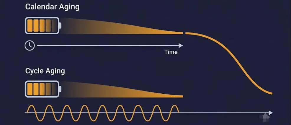
Battery Degradation in BESS: Causes, Mechanisms & Mitigation
Every battery energy storage system loses capacity over time. That process, battery degradation in BESS, is not a flaw. It is a normal part of how lithium-ion cells age. So the real question is not whether battery degradation happens. It is how fast, and how much control you have over the rate.
This guide breaks down what drives battery degradation in BESS, across grid-scale and commercial LFP systems. First, it covers what happens inside the cell. Then it covers which choices slow the process down. It also links to deeper guides on each mechanism, so you can go as deep as you need.
| Quick Answer Battery degradation in BESS is the slow, permanent loss of usable capacity and rise in internal resistance. Two things drive it. Calendar aging happens with time and is worst at high state of charge. Cycle aging happens from charging and discharging. Heat speeds up both. |
What Is Battery Degradation in BESS?
Battery degradation in BESS shows up as two signs. First, the battery holds less energy than it did when new. Second, its internal resistance goes up. So more energy is lost as heat during use.
Both signs share one root cause. Lithium ions get used up by side reactions instead of doing real work. Some get trapped in a growing layer on the anode. Then others get lost when the electrode structure breaks down. So once a lithium ion is lost, that capacity does not come back.
For LFP systems, the news is fairly good. A well-run, grid-scale LFP battery typically loses 20% to 30% of its capacity over ten years. But numbers like these take real operating discipline. They do not happen by luck.
Two Degradation Pathways: Calendar Aging vs. Cycle Aging
Every BESS ages through two paths at once.
Calendar Aging
Calendar aging happens purely with time. Then it keeps going even while a battery sits idle. State of charge is the biggest driver. Temperature is a close second. So cells stored at high state of charge age faster, especially above 80%.
Cycle Aging
Cycle aging comes from charging and discharging. Also, it scales with cycle count, discharge depth, and charge rate. But use temperature matters too. A battery run hard at high current takes more stress per cycle than one run gently.
Field data backs this up. Tests on large-format LFP cells built for stationary storage found something clear. Temperature has the biggest effect on aging. Still, the cycling pattern matters less by comparison. So thermal management should come first in any BESS design.
For a deeper look at how to split these two effects in real data, see our full guide on Calendar Aging vs. Cycle Aging in LFP Batteries.
What’s Happening Inside the Cell: SEI Growth and Lithium Plating
Battery degradation in BESS is at its core a chemistry problem. Two mechanisms cause most of the damage inside an LFP cell.
The first is growth of the solid electrolyte interphase, or SEI. This is a thin layer that forms on the anode surface. Also, some SEI growth is normal, even needed at first. Yet it keeps growing slowly over the battery’s life. Each time it thickens, it uses up lithium ions and electrolyte. At high state of charge, SEI growth speeds up. Then that growth also raises internal resistance. So aging cells run hotter and less efficiently than new ones.
The second mechanism is lithium plating. Instead of moving cleanly into the anode, lithium ions build up as metal on the surface. First, this mostly happens during fast charging in cold weather. Then the anode simply cannot take in lithium fast enough. So plated lithium is mostly lost capacity for good. In bad cases, it can also raise safety risks.
Both mechanisms show why how you charge matters as much as how much. For the full picture, read our guide on SEI Layer Growth and Lithium Plating in LFP Cells.
Temperature’s Outsized Role in Battery Degradation in BESS
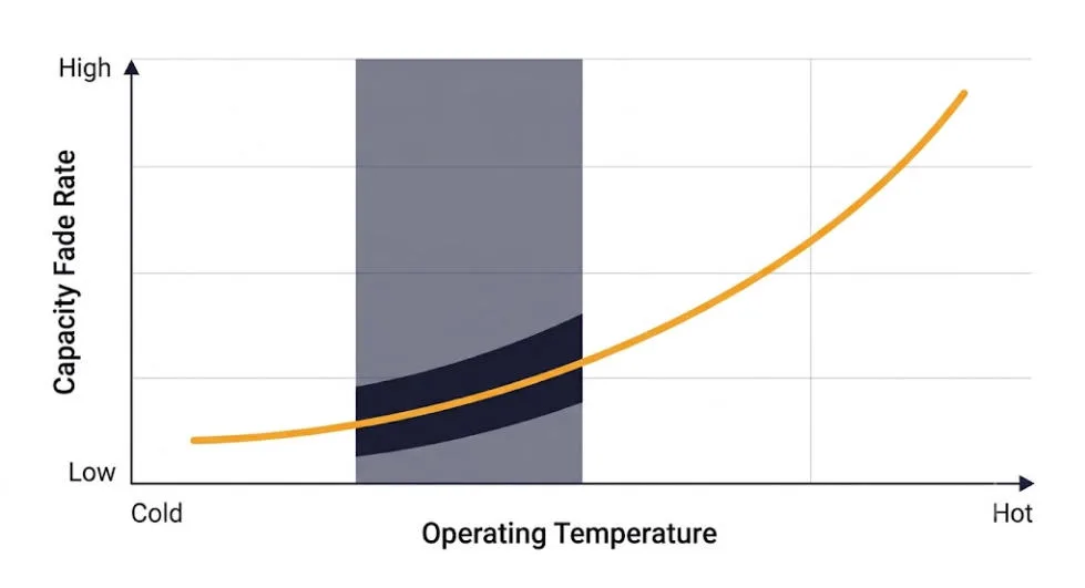
One factor beats every other factor: temperature. Heat speeds up SEI growth. It speeds up calendar aging. Also, it raises the rate of unwanted side reactions across the board. This holds true whether the battery sits idle or runs hard.
Cold brings a different problem. First, below a certain point, an LFP cell cannot take a charge quickly. Fast charging in the cold pushes cells toward the plating risk covered above. This is a design issue, not just a chemistry issue. So it shapes everything from enclosure size to winter charge-rate limits.
This section covers the general heat effect. If you run a system in a cold climate, our guide on Cold-Climate BESS Design covers cutoff behavior in full detail. For the underlying temperature/cycle-life relationship, see our existing guide, Impact of Temperature on LiFePO₄ Batteries Cycle Life. For the underlying mechanism behind why heat and cold both accelerate degradation, see our guide on How Temperature Accelerates Battery Degradation: The Arrhenius Relationship.
Operating Choices That Speed Up or Slow Down Degradation
Battery degradation in BESS is not fully out of your hands. Several choices have a direct, real effect on how fast it happens.
Depth of Discharge and C-Rate
First, deeper discharges add more stress per cycle than shallow ones. But they also deliver more usable energy, so there is a real tradeoff. So many operators run at 0.5C or lower to cut this stress. Still, going past 80% discharge depth often adds up over thousands of cycles.
State of Charge Operating Window
High state of charge speeds up calendar aging through faster SEI growth. Very low state of charge, below about 20%, brings a different risk. Also, it can dissolve current collectors and weaken the electrode. So most operators keep cells inside a 20% to 80% band. So they skip the full 0% to 100% range in daily use.
For the full breakdown of how these variables interact at the particle level, read our guide on Why Deep Discharge and High C-Rate Stress LFP Cells.
Tracking Battery Degradation in BESS: State of Health Estimation
You need a solid way to track battery degradation in BESS before you can manage it. That is harder for LFP cells than for most other chemistries.
LFP cells have a nearly flat voltage curve across the 20% to 80% state-of-charge range. So voltage barely moves across that wide middle band. So voltage-based tracking is not reliable on its own. LFP cells also show hysteresis. Also, voltage during charge and discharge differs by roughly 5 to 25 millivolts at the same state of charge. So both quirks make simple voltage checks a poor tool for tracking degradation.
Coulomb counting is the most common baseline method. It skips the voltage problem, but it still drifts over time from small sensor errors. But left alone, that drift adds up across thousands of cycles. So better systems add regular recalibration. But some also track internal resistance. Still others use model-based tools like an Extended Kalman Filter to keep the estimate honest as cells age.
This ties right into your BMS. For the full comparison of methods, see our guide on BMS SOC Estimation Methods Explained. For a closer look at tracking degradation itself, read Advanced SOH Estimation for BESS.
How to Slow Battery Degradation in BESS: A Practical Summary
| Strategy | Why It Helps |
| Keep SOC in a 20-80% operating band | Cuts both calendar aging and low-SOC electrode stress |
| Manage temperature actively | Temperature is the top driver of aging in most studies |
| Limit fast charging in cold weather | Cuts lithium plating risk at the anode |
| Avoid needless deep discharges | Cuts mechanical and chemical stress per cycle |
| Track SOH with more than coulomb counting alone | Catches drift before it skews dispatch decisions |
| Recalibrate BMS capacity estimates often | Keeps SOC and SOH readings accurate as cells age |
Frequently Asked Questions
How much does a BESS degrade per year?
A well-run, grid-scale LFP system typically loses 20% to 30% of its capacity over ten years under good operating conditions. Fade is not perfectly linear year to year, so treat this as a decade-scale range rather than a fixed annual number.
What causes the most battery degradation in BESS?
Temperature and state of charge are the two biggest drivers, by far. High temperature speeds up nearly every aging mechanism at once. High state of charge speeds up calendar aging too, even when the battery sits idle.
Does battery degradation in BESS ever stop?
No. Degradation is steady and permanent. Good thermal management and SOC discipline can slow it a lot. But nothing stops it entirely.
Is LFP more resistant to degradation than other lithium-ion chemistries?
Yes. LFP is more stable than nickel-based chemistries like NMC. That is a big reason it leads in stationary storage. It still degrades, just more slowly and more predictably under the same conditions.
Further Reading
Calendar Aging vs. Cycle Aging in LFP Batteries
Advanced SOH Estimation for BESS
SEI Layer Growth and Lithium Plating in LFP Cells
How Temperature Accelerates Battery Degradation: The Arrhenius Relationship
Why Deep Discharge and High C-Rate Stress LFP Cells
BMS SOC Estimation Methods Explained: OCV vs Coulomb Counting vs Kalman Filter
Cold-Climate BESS Design: Discharge-Side DCIR and Premature Cutoffs
Cold-Climate BESS Design: Discharge-Side DCIR and Premature Cutoffs
Most cold-weather BESS design attention goes to charging. Lithium plating below roughly 0°C is a real, well-documented risk. Charge-inhibit logic is standard practice for good reason. Discharge-side cold behavior gets far less coverage. But it drives a different problem: resistance-driven voltage sag that trips a cutoff long before the pack is actually empty. This guide covers cold-climate BESS design for the discharge side specifically. It covers how cold amplifies the same DCIR mechanism covered in our dynamic cutoff design guide. It also covers what that means for current de-rating, heater sizing, and enclosure insulation.
| ⚡ Quick Answer Cold-climate BESS design has to account for LFP internal resistance rising sharply as temperature drops, since ion mobility slows in the electrolyte and at the electrode interface. This increases voltage sag under load, which can trip a fixed or even a DCIR-adaptive cutoff early if the resistance lookup table doesn’t extend to true cold-climate minimums. The design response has three parts: extending the cutoff’s temperature matrix to cover real winter conditions, applying current de-rating as temperature drops, and sizing enclosure heating and insulation to keep cells out of the steepest part of the resistance curve. |
Why Cold-Climate BESS Design Needs to Address Discharge-Side DCIR
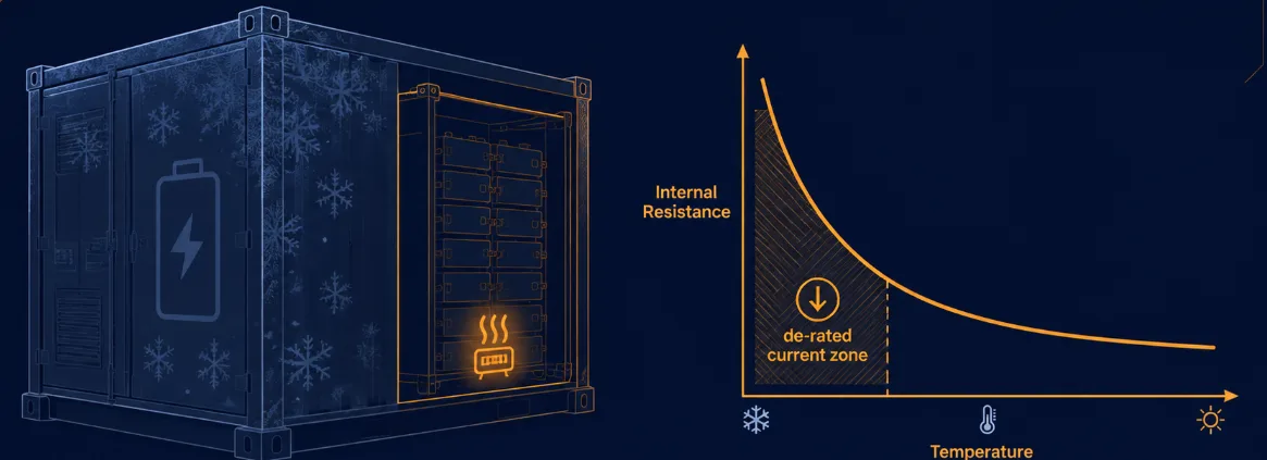
Our DCIR-adaptive cutoff design guide covers how internal resistance rises with cell age. It also covers how a fixed cutoff voltage fails to account for that rise. Cold temperature drives the same mechanism through a different cause. As temperature drops, electrolyte viscosity increases and ionic mobility slows, both in the bulk electrolyte and at the electrode interface. That raises internal resistance independent of cell age or cycle count. A fresh cell at -10°C can show meaningfully higher resistance than an aged cell at 25°C.
The practical effect is the same voltage-sag mechanism covered in the cutoff design guide.
Vterminal = VOCV − I × DCIR
A higher DCIR term means more sag at identical current, which reaches a fixed trip voltage sooner. This isn’t a marginal effect. A coupled electrochemical-thermal model validated against real cells from -20°C to 45°C confirms resistance rises sharply as temperature drops. Usable discharge capacity falls well below nameplate rating in the -10°C to -20°C range. That drop is driven primarily by the resistance rise, not by any real loss of stored charge. The energy is still in the cell. The pack just can’t deliver it fast enough to clear the cutoff threshold at typical discharge rates.
This matters most for anyone who has already implemented a DCIR-adaptive cutoff per our earlier guide. Say the HPPC test matrix behind that lookup table stopped at a moderate low-temperature bound, rather than the site’s true winter minimum. In that case, the adaptive cutoff extrapolates poorly. It can even fail safe into overly conservative behavior — exactly in the conditions where it matters most.
Extending the Cutoff Matrix for Cold-Climate BESS Design
The fix is directly upstream of implementation, not a separate system. The HPPC test campaign behind a DCIR-adaptive cutoff needs a temperature range that matches real deployment conditions. It shouldn’t just reflect a generic qualification range. A system specified for a temperate climate, but deployed somewhere with regular sub-zero winter lows, needs its lookup table re-tested. It needs to be rebuilt for that colder range. That should happen before commissioning, not patched in after a field failure.
Two practical points from that testing process carry directly into cold-climate design:
- Pulse-test resistance at temperature steps that bracket the real minimum with margin, not just the design spec’s stated floor. Local weather can exceed nameplate assumptions during extreme events.
- Re-validate hysteresis settings at cold temperature specifically. A cutoff tuned for hysteresis behavior at room temperature can behave differently at the steeper part of the resistance curve. There, small current fluctuations produce larger voltage swings.
Current De-Rating Strategy for Cold-Climate BESS Design
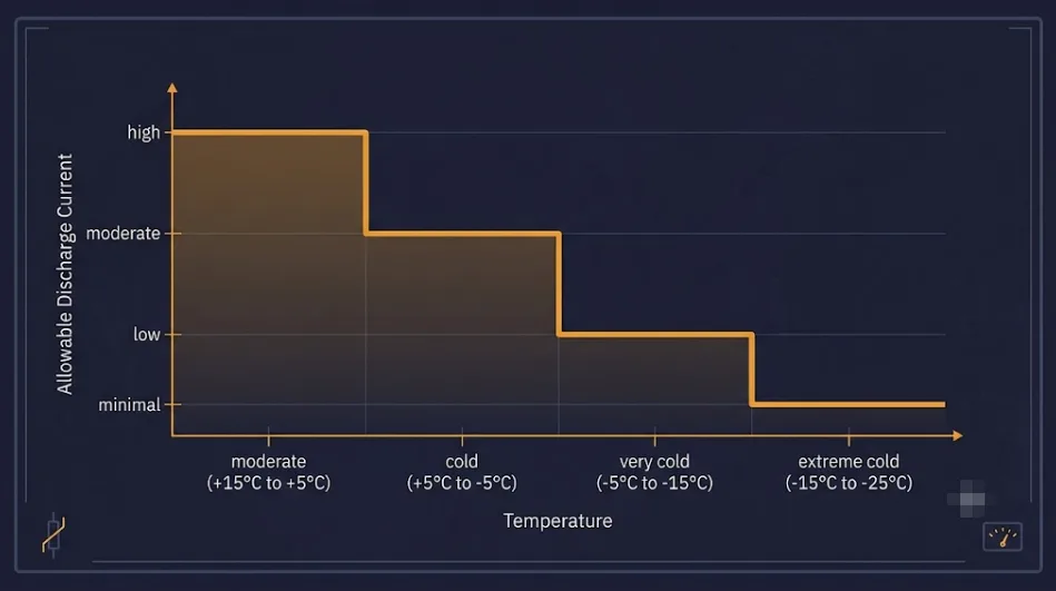
Even with an accurate cold-temperature resistance map, discharging at full rated current in cold conditions is risky. It pushes the system into the steepest part of the resistance curve. That’s where voltage sag grows fastest per unit of additional current. Current de-rating reduces the maximum allowed discharge current as measured cell temperature falls. It keeps the operating point away from that steep region. That’s safer than relying on cutoff logic alone to catch the problem after the fact.
A practical de-rating curve ties allowable current to the same temperature bands used in the DCIR lookup table. It steps down current limits at each band, rather than applying one blanket reduction across the entire cold range. This preserves as much usable power as safely possible at moderately cool temperatures. It pulls back harder as conditions approach the pack’s true low-temperature floor.
Heater Sizing for Enclosure Thermal Management
Where current de-rating manages the symptom, enclosure heating addresses the cause. It keeps cells out of the steep-resistance temperature range in the first place. A Sandia-led modeling study across eight U.S. locations found that enclosure heating and cooling loads alone increased required battery energy capacity. The increase ranged from 42% to 300%, depending on climate severity. The same study found that power conversion system placement matters too. Keeping the PCS inside the thermally managed envelope reduced the capacity penalty; leaving it exposed outside increased it. That model was built around an NMC cell, not LFP. LFP chemistry is generally more resistance-sensitive in cold conditions. So the real capacity penalty for an LFP system is likely at or above this range, not below it.
Heater sizing follows standard enclosure thermal design practice. Calculate steady-state heat loss for the enclosure’s surface area and target ΔT. Then apply a safety margin, commonly in the 125–130% range. That covers thermal mass and startup transients, not just steady-state loss. Insulation quality changes this calculation substantially. A well-insulated enclosure can cut steady-state heat loss by roughly 90% compared to an equivalent bare-metal enclosure. That’s normally the larger lever before reaching for a bigger heater.
Insulation and Enclosure Strategy in Cold-Climate BESS Design
BESS enclosures almost always use sealed-loop climate control rather than direct outside-air ventilation. Pulling ambient air through the battery compartment introduces humidity, salt, and dust. Those contaminants degrade cells and can create insulation-resistance faults over time. A cold-climate site often adds condensation risk too, from indoor-outdoor temperature swings. The standard architectures are a split air-conditioning unit with a sealed evaporator inside the compartment, for small to mid-size systems. Larger systems, above roughly 1 MWh or with high C-rate demands, typically use liquid cooling with cold plates instead. Whichever architecture is used, insulation determines how hard the heater has to work. It’s what holds the compartment above the steep-resistance zone, making it a critical factor in overall cold-climate BESS design. That’s worth specifying to the actual climate data for the site, not a generic regional assumption.
Bringing It Back to the Cutoff and Estimation Layers
Cold-climate design doesn’t introduce a new subsystem. It extends the temperature range that two subsystems already covered in this series need to handle correctly. The DCIR-adaptive cutoff’s lookup table needs a temperature axis that reaches the site’s true minimum. An EKF-based SOC estimator built from the same HPPC campaign needs its equivalent circuit model fitted across that same cold-temperature range. A model that only saw moderate temperatures during characterization will estimate poorly outside that range. Our EKF SOC estimation design guide and DCIR-adaptive cutoff design guide both assume the underlying test matrix covers real operating conditions. Cold-climate deployment is where that assumption needs the most scrutiny.
Key Takeaways
Cold-climate BESS design starts with the same electrolyte-viscosity and ion-mobility mechanisms that raise LFP internal resistance with age. That resistance rise produces the same voltage-sag effect that drives premature cutoffs. A DCIR-adaptive cutoff only protects against this if its HPPC test matrix extends to the site’s real winter minimum. A generic qualification range isn’t enough. Current de-rating tied to temperature bands keeps the operating point out of the steepest part of the resistance curve. That’s safer than relying on cutoff logic alone. Enclosure heater sizing should follow standard steady-state-plus-safety-margin methodology, with insulation quality as the larger lever before increasing heater capacity. Cold-climate design extends the same estimation and cutoff systems covered elsewhere in this series, rather than requiring a separate architecture.
Frequently Asked Questions
Does a DCIR-adaptive cutoff automatically handle cold-climate conditions?
Only if the HPPC test matrix used to build its lookup table extends to the site’s real winter minimum temperature. A table built against a generic or moderate qualification range will extrapolate poorly at true cold-climate lows. That can produce either an unsafe cutoff or an overly conservative one.
Is current de-rating necessary if the enclosure is heated?
Even a well-heated enclosure has a startup period. It can also see localized cold spots before reaching steady state. Current de-rating remains a useful safeguard during that transition. It’s not made redundant by heating alone.
How much does insulation actually reduce heater size?
A well-insulated enclosure can cut steady-state heat loss by roughly 90% compared to an equivalent bare-metal enclosure. That’s typically a larger lever than increasing heater wattage on a poorly insulated design.
References
Ji, Zhang, Wang — “Li-Ion Cell Operation at Low Temperatures,” Journal of The Electrochemical Society (2013)
Sandia National Laboratories / Energy journal — Impact of Heating and Cooling Loads on Battery Energy Storage System Sizing in Extreme Cold Climates
Further Reading
Dynamic, DCIR-Adaptive Voltage Cutoff Design for LFP BESS
EKF SOC Estimation Design for LFP BESS
Designing an LFP BESS Against SOC Drift, Cell Imbalance, and Premature Cutoffs