
Earthing (Grounding) for a Battery Energy Storage System (BESS): A Complete Design Guide
A BESS grounding system ties every battery rack, enclosure, and steel structure back to a common earth point. So, when a fault happens, current gets a fast path home. But get the BESS grounding system wrong, and one insulation fault can turn a cabinet into a shock hazard. It can also start a slow fire risk. So this guide covers the earthing methods, code rules, and design steps that keep a battery storage site safe. First, it covers soil testing. Then it covers ground grid sizing.
| Quick Answer A BESS grounding system bonds every metal part of a battery storage site to a common earth reference. Earthing is the term IEC-based countries use. Grounding is the U.S. term. But both mean the same thing. In the U.S., NEC Article 706 sets the rules for systems above 50V AC or 60V DC. Meanwhile, most other countries follow IEC 60364 instead. That standard defines TN, TT, and IT earthing systems. Also, a strong BESS grounding system needs a buried grounding electrode system. Many modern DC buses add high-resistance grounding too. So an insulation monitoring device watches for faults, instead of a solid ground wire alone. |
Why a BESS Grounding System Matters
Grounding is not paperwork. Instead, it decides whether a fault trips a breaker in milliseconds. Or, it decides whether a fault energizes a cabinet a technician is standing next to. A BESS site packs high fault current into a small footprint. Also, workers open enclosures often for maintenance. So the margin for error stays thin.
Personnel Safety
A bonded enclosure stays close to earth potential during a fault. But without that bond, a failure inside a battery cabinet can raise the metal casing to a dangerous voltage. Then anyone touching it completes the circuit. So this is the core safety case behind every BESS grounding system, at any project size.
Equipment and Fire Protection
A fast, low-impedance fault path lets breakers clear a ground fault quickly. Otherwise, the fault can grow into an arcing fault. And arcing near lithium-ion cells is a real ignition risk.
Our BESS short-circuit protection guide covers that risk in detail. So a sound BESS grounding system and short-circuit protection work as one safety strategy, not two separate items.
Protective-Device Coordination
Relays and fuses only work as fast as the fault path allows. But a weak ground path slows fault detection down. As a result, a fault can stay energized far longer than planned. So grounding design and protection coordination need to be solved together.
Earthing vs. Grounding: Same Idea, Different Vocabulary
Earthing and grounding name the same practice. First, IEC-based markets say earthing. That includes the UK, the EU, Australia, and most of Asia. Then, NEC-based markets say grounding. The United States is the main example. Still, both terms mean bonding conductive parts to earth for safety. So this guide uses both terms, matching whichever code applies to a given project.
Codes and Standards Behind a BESS Grounding System
No single global code covers earthing for battery storage. Instead, a BESS grounding system usually has to satisfy several overlapping standards. So the table below summarizes the main ones.
| Standard | Region | What It Covers |
|---|---|---|
| NEC (NFPA 70) Article 706 | United States | Covers permanently installed ESS above 50V AC or 60V DC. Sets bonding, disconnect, and circuit-protection rules |
| IEC 60364 | International | Defines TN, TT, and IT earthing system classes for low-voltage installations |
| IEEE Std 80 | International reference | Guide for AC substation grounding. Sets step- and touch-voltage limits for larger ground grids |
| IEEE Std 142 (Green Book) | International reference | General power-system grounding practice, covering equipment and system grounding |
| NFPA 855 | United States | ESS siting and spacing, which pairs with grounding design |
For example, NEC Article 706 sets the U.S. baseline for a BESS grounding system. Also, our NFPA 855 guide covers the fire-code side of siting and spacing. Meanwhile, lightning protection sits alongside a BESS grounding system, not inside it. We cover that later in this guide.
NEC Article 706’s scope line matters most for design choices. So it applies to any permanently installed ESS above 50V AC or 60V DC. That covers nearly every commercial and utility-scale BESS grounding system built today.
Types of Earthing Systems in a BESS Grounding System
TN, TT, and IT Systems (IEC 60364)
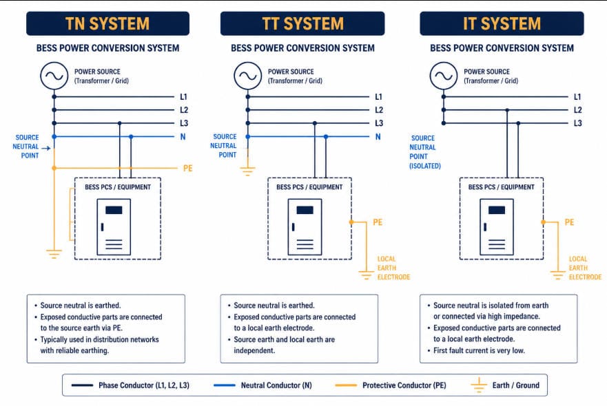
IEC 60364 uses a two-letter code for each earthing system. First, the first letter shows how the source relates to earth. Then, the second shows how equipment is earthed. TN systems bond equipment to the source’s earthed neutral. So that gives fast fault clearance through ordinary breakers. TT systems instead use a separate, independent earth electrode at the site. They rely on residual-current devices to catch smaller faults. IT systems isolate the source from earth, or use high impedance instead. So this favors continuity of supply over instant clearance. It is a common choice for critical DC sections.
See this IEC 60364 earthing system overview for the full classification breakdown.
Solidly Grounded, Ungrounded, and High-Resistance Grounded DC Buses
The battery-side DC bus needs its own decision, separate from the AC earthing system. First, older, PV-derived designs often grounded the DC bus solidly. Then a ground-fault detector-interrupter opened the bond on a fault. Today, many modern, transformerless power conversion systems instead run the DC bus ungrounded or high-resistance grounded. So an insulation monitoring device watches it continuously, instead of a fuse-based interrupter. The table below compares all three approaches.
| Approach | Fault Detection | Typical BESS Use |
|---|---|---|
| Solidly grounded | Fast — an overcurrent device clears the fault path directly | Legacy PV-battery hybrids, some low-voltage residential or C&I designs |
| Ungrounded (floating) | Continuous insulation-resistance monitoring, no automatic first-fault trip | Modern transformerless PCS topologies where uptime matters most |
| High-resistance grounded | Limits fault current while a monitoring device flags the fault | Utility-scale strings and central PCS designs balancing safety and uptime |
This choice depends heavily on PCS topology. So it belongs in the same conversation as PCS overvoltage protection and grid-forming versus grid-following control. It should never be bolted on after the fact.
Core Components of a BESS Grounding System
Equipment Grounding and Bonding in a BESS Grounding System
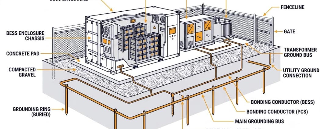
Every metal enclosure, rack, and structural part needs a bonding jumper. That jumper must reach back to the grounding system. Also, it needs to be sized for the worst-case fault current. First, painted surfaces need a bare-metal bonding point, since paint is an insulator. Also, fence gates and conduit expansion joints need flexible jumpers, so thermal movement never breaks continuity.
Conductor size follows the code, not a guess. So the table below gives quick reference points for both major code families.
| Reference | Basis | Quick Rule |
|---|---|---|
| NEC Table 250.66 (GEC sizing) | Size of the largest ungrounded service conductor | A GEC run solely to a rod, pipe, or plate electrode never needs to exceed 6 AWG copper |
| NEC Table 250.122 (EGC sizing) | Rating of the upstream overcurrent device | Equipment grounding conductors scale with breaker or fuse size, not with the circuit conductor size |
| IEC 60364-5-54 (PE sizing) | Cross-sectional area of the phase conductor | PE equals the phase size up to 16 mm², stays at 16 mm² up to 35 mm², then drops to half the phase size above that |
The Grounding Electrode System
This is the buried hardware that gives fault current a path into the earth. It can be ground rods, a ground ring, or a full mesh grid. So, site size drives the choice. First, a small C&I rooftop or pad-mounted BESS can use a simple rod-based electrode system. Then, a utility-scale site instead needs a buried copper mesh grid. That grid must meet IEEE 80 step- and touch-voltage limits.
Grounding a Containerized or Mobile BESS
Containerized and trailer-mounted BESS units add a wrinkle. Often, they sit on gravel, asphalt, or a temporary pad, not poured concrete. So a concrete-encased electrode is rarely an option there. Instead, crews drive temporary ground rods, or lay a portable ground mat, at each deployment site. Also, every container or trailer section needs a bonding strap back to that temporary electrode, plus jumpers between linked sections. Since soil conditions change from site to site, resistance needs a fresh test at every new location, not just once back at the factory.
DC Ground-Fault Detection and Insulation Monitoring
On the DC side, ground-fault detector-interrupters and insulation monitoring devices solve the same problem in different ways. Both catch a fault between a live conductor and ground before it becomes an arc. Also, an insulation monitoring device measures leakage resistance continuously. So it raises an alarm well before resistance drops to a dangerous level. That is why it has become the default choice on ungrounded and high-resistance grounded DC buses.
Avoiding Ground Loops in a BESS Grounding System
Power grounding is not the only ground reference on a BESS site. Comms wiring also needs care. That includes CAN bus, RS-485, or IEC 61850 links between racks, the BMS, and the PCS. So a shielded comms cable should bond to ground at one end only. Otherwise, bonding both ends creates a ground loop. Then, even a small voltage difference between the two ground points drives current through the shield. That current, in turn, induces noise onto the signal pair. Common symptoms include noisy cell-voltage readings, checksum errors, and comms dropouts, especially during heavy charge or discharge events. So plan single-point grounding for comms at design time, not after commissioning turns up faults.
Designing a BESS Grounding System’s Electrode Network
Soil Resistivity Testing
Soil resistivity, not conductor size, drives ground rod performance the most. It shifts with moisture, temperature, and soil type. So a resistivity survey should happen early in site design, not after the rods are already buried. The four-pin Wenner method is the standard test. Also, sandy or rocky soil can carry resistivity several times higher than loam. That directly raises the rod count, the grid area, or the need for ground-enhancement material.
The Concrete-Encased Electrode (Ufer Ground)
Most C&I and utility-scale BESS pads already sit on poured concrete. So that concrete can double as a grounding electrode. NEC 250.52(A)(3) allows this. A concrete-encased electrode, often called a Ufer ground, uses at least 20 feet of rebar or bare copper conductor, encased in at least 2 inches of concrete that touches the earth. Since a Ufer ground typically beats a driven rod on resistance, especially in dry or rocky soil, it is worth planning before the pour, not after. Once the concrete cures, adding one later means breaking into a finished pad.
Worked Example: Sizing Ground Rods for a C&I BESS Pad
Take a standard 8-foot, 5/8-inch copper-clad ground rod. Place it in average loam soil, with a resistivity of 100 Ω·m. Using the standard single-rod resistance formula, that rod works out to roughly 40 Ω. So that is above the 25 Ω threshold NEC 250.53(A)(2) sets for a single rod, pipe, or plate electrode. Then, a second rod, spaced at least 6 feet away, usually brings the combined resistance under that 25 Ω limit. But mutual interference between rods means the drop is never a clean 50%. In high-resistivity ground — sandy or rocky soil at 300 Ω·m or more — a single rod can exceed 100 Ω. There, the fix shifts from adding rods to a driven ground ring, chemical rods, or ground-enhancement backfill.
Step and Touch Voltage for Utility-Scale Sites
Larger sites need more than a resistance number. So IEEE Std 80 sets tolerable step- and touch-voltage limits. These depend on soil resistivity, fault-current size, and clearing time. Then, the standard works backward to the mesh spacing a ground grid needs. Still, a grid can show low overall resistance and still fail an IEEE 80 check. That happens when the voltage gradient across the grid surface runs too steep. So resistance alone is never the full design target for a utility-scale BESS grounding system.
See this IEEE Std 80 grounding interpretation for the underlying safety criteria.
Lightning Protection Sits Alongside Earthing
Lightning protection systems use their own down-conductor and electrode network. NFPA 780 covers this in the U.S. IEC 62305 covers it internationally. So this network is engineered for high-frequency surge current. It stays distinct from the power-system grounding electrode system. Still, the two networks are typically bonded together at grade. That prevents a dangerous potential difference between them during a strike.
Surge protective devices on the AC and DC sides, covered in our PCS overvoltage protection guide, round out the site’s full surge coordination plan.
Common BESS Grounding System Mistakes
- Treating a painted enclosure surface as a bonding point, instead of scraping to bare metal first.
- Installing a single ground rod without testing resistance, then assuming it clears the NEC 25 Ω threshold.
- Skipping flexible bonding jumpers across fence gates and conduit joints, which breaks continuity as materials move.
- Solidly grounding a DC bus on a transformerless PCS without checking manufacturer guidance, which can cause nuisance trips.
- Sizing a ground grid to a resistance target alone, with no IEEE 80 step- and touch-voltage check on a utility-scale site.
- Bonding bare copper directly to galvanized steel rebar or racking in humid or coastal soil, which speeds up galvanic corrosion at the connection point.
- Never re-testing soil resistivity or ground resistance after commissioning, even though seasonal moisture changes both.
Key Takeaways
- A BESS grounding system bonds every conductive part to a common earth reference. That gives fault current a defined, low-impedance path home.
- NEC Article 706 governs U.S. installations above 50V AC or 60V DC. IEC 60364’s TN, TT, and IT classes govern most other markets.
- Many modern, transformerless PCS designs run the DC bus ungrounded or high-resistance grounded. An insulation monitoring device watches it instead of a solidly grounded fuse-based interrupter.
- A single ground rod in average soil rarely meets NEC’s 25 Ω threshold alone. Test soil resistivity before the rods go in the ground, not after.
- A poured concrete BESS pad can double as a Ufer ground under NEC 250.52(A)(3), often beating a driven rod on resistance in dry or rocky soil.
- Keep comms shields single-point grounded. Bonding both ends of a CAN bus, RS-485, or IEC 61850 shield creates a ground loop that shows up as noisy readings and comms dropouts.
- Utility-scale sites need an IEEE 80 step- and touch-voltage check. A low resistance reading alone does not guarantee a safe voltage gradient.
- Lightning protection and power-system grounding are separate networks. Bond them together at grade; do not treat them as one system.
- Grounding design, short-circuit protection, and overvoltage protection form one coordinated safety strategy, not three separate checklists.
Frequently Asked Questions
Does the NEC Require a BESS Grounding System?
Yes. For any permanently installed ESS above 50V AC or 60V DC, NEC Article 706 sets bonding, disconnect, and circuit-protection rules. These form the core of a compliant BESS grounding system.
What Ground Resistance Does a BESS Grounding System Need?
The NEC benchmark for a single rod, pipe, or plate electrode is 25 Ω or less. If one rod misses that mark, add a supplemental rod at least 6 feet away. Utility-scale sites also need an IEEE 80 step- and touch-voltage check, on top of a lower target resistance.
Should a BESS DC bus be grounded or ungrounded?
It depends on the PCS topology. Many modern, transformerless designs use an ungrounded or high-resistance grounded DC bus with continuous insulation monitoring. Some legacy or transformer-based designs still solidly ground the bus with a ground-fault detector-interrupter. Follow the PCS manufacturer’s guidance rather than a default assumption.
Does a Containerized or Mobile BESS Need Different Grounding?
Yes, somewhat. A fixed pad lets a BESS grounding system use a concrete-encased electrode. A mobile or trailer-mounted unit usually cannot rely on that. So it needs temporary ground rods or a portable ground mat at each site, plus fresh resistance testing every time it moves.
How often should a BESS grounding system be tested?
Test ground resistance and bonding continuity at commissioning first, using a fall-of-potential test or a clamp-on ground resistance tester. Then, re-test on a regular maintenance schedule. Soil resistivity shifts with seasonal moisture and temperature, so a compliant reading at commissioning can drift over time.
Further Reading
- BESS Short Circuit Protection
- PCS Overvoltage Protection
- Understanding BESS Specifications
- NFPA 855 Guide
- LVRT and HVRT Ride-Through
- Grid-Forming vs. Grid-Following BESS
- BESS PCS Functions and Features
- NEC Article 706 overview (up.codes)
- IEEE Std 80 substation grounding interpretation (standards.ieee.org)
- IEC 60364 earthing system classification overview (ecalpro.com)
BESS Augmentation: AC Block Addition vs. DC Shuffling — How Mid-Life Capacity Upgrades Actually Work
AC block addition is one of two ways to carry out BESS augmentation. BESS augmentation, in short, restores capacity a battery loses over time. Every charge and discharge cycle wears the cells down. So, after a few years, the system can no longer deliver its full contracted energy or power. AC block addition fixes this by adding new inverters and battery racks on the AC side. DC shuffling, the other path, instead reallocates existing modules behind the inverters already on site. Each approach, however, solves the same problem differently.
| Quick Answer AC block addition installs a new, independent power block behind its own connection point. It costs more and needs more space. However, it works with any battery chemistry, and it skips synchronization headaches with old cells. DC shuffling, by contrast, reorganizes and adds battery modules behind the existing inverters. It costs less, and it often avoids new interconnection permits. But busbar ratings, breaker capacity, and voltage matching all limit how much capacity it can add. |
Why BESS Augmentation Needs a Capacity-Adding Strategy
This guide focuses on the technical mechanics of the two paths. For the full picture on BESS augmentation as a strategy, including how it compares to oversizing capacity upfront, see our BESS Augmentation: The Complete Guide.
Lithium-ion cells degrade with use. So does calendar time alone. Each cycle stresses the electrode material. Specifically, the protective SEI layer on the anode cracks and reforms. This, in turn, consumes active lithium every time. High charge rates and cold temperatures make it worse.
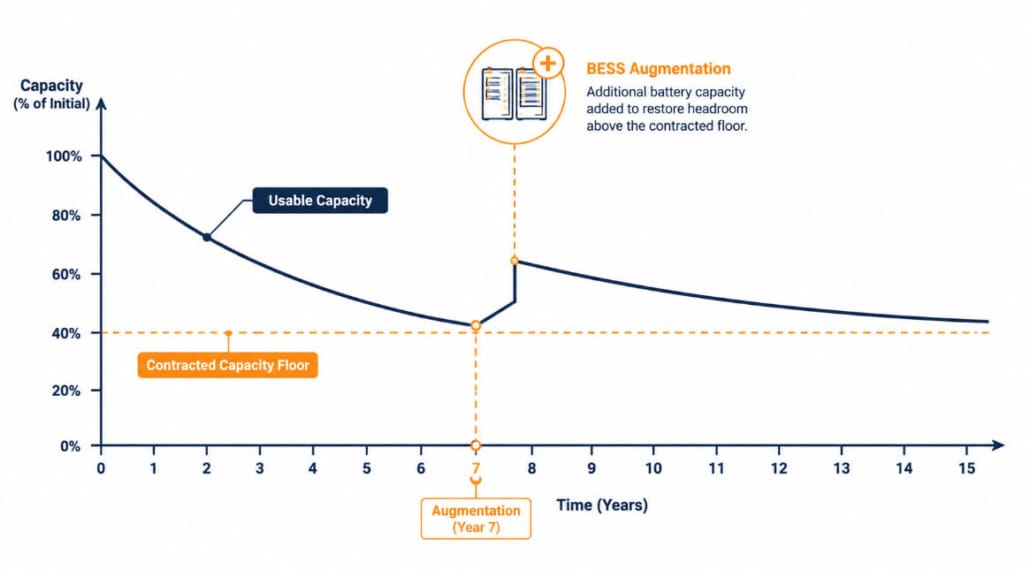
Fade rates vary by chemistry and duty cycle. Many grid-scale LFP systems, for instance, lose roughly 2 to 3 percent of usable capacity per year. As a result, after five to seven years, a project can fall short of its contracted energy or power. That, in turn, threatens revenue under tolling agreements and capacity contracts.
BESS augmentation exists to close that gap. It adds capacity back, either instead of, or alongside, overbuilding extra capacity at day one. Modo Energy’s research on the topic frames it simply: augmentation restores or increases capacity, and both outcomes improve a project’s revenue potential.
Cycle Aging and the Restore Buffer
BESS augmentation is not a one-time fix. Instead, most projects restore capacity to a buffer above nameplate, not just back to nameplate. That buffer, in turn, gives headroom before the next augmentation cycle is needed.
Here is the catch. That buffer is defined in AC terms, at the point of interconnection. See our guide to understanding BESS specifications for how nameplate, usable, and contracted energy differ. But the actual work is a DC decision, since operators install battery cells, not AC megawatts. So, converting between the two requires accounting for round-trip losses across the inverter and transformer.
AC Block Addition Explained
How the AC Path Works
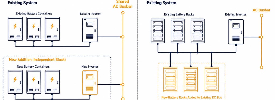
AC block addition adds a self-contained power block next to the existing system. New battery racks, a new PCS, and often a new transformer, arrive as one unit. The block then synchronizes independently at the AC bus, or at a new point of interconnection. Because the new block does not share a DC bus with old batteries, voltage and state-of-charge mismatches between aged and fresh cells never become a problem.
Pros and Cons of the AC Path
Advantages:
- Works with any battery chemistry — operators can add a sodium-ion or next-generation LFP block next to an aging system.
- Needs no voltage or state-of-charge synchronization with degraded cells.
Offers a chance to upgrade PCS technology, such as adding grid-forming capability, alongside the capacity add.
- Creates a clean equipment and warranty boundary between old and new hardware.
Drawbacks:
- Costs more, since a new PCS, transformer, and switchgear all add expense.
- Needs more physical footprint.
- Often triggers a new interconnection study or re-permitting, since new grid-connected hardware is involved.
Adds a new fault-current source, so protection settings must be re-coordinated.
DC Shuffling Explained
DC shuffling reorganizes existing battery modules behind the inverters already in service. Modules with similar degradation profiles get grouped together. This, in turn, spreads energy more evenly across the stack. On its own, however, shuffling does not add any capacity. It just rebalances what is already there.
Real capacity gets added only when new racks are added behind the same PCS, after the existing fleet has been shuffled and rebalanced. Because the new capacity shares the existing inverter and bus, the project may be able to avoid a new grid interconnection point. However, permitting and approval requirements still depend on the scope of the modification and the applicable jurisdiction. A DC-to-DC converter can help reconcile the voltage gap between old and new modules. The converter itself, though, adds no capacity on its own.
Technical Limits of DC Shuffling
DC shuffling looks cheap on paper. However, it runs into hard technical ceilings. As Energy-Storage.News has reported, auxiliary load breakers and busbars were sized for the original system. So, adding capacity behind them can exceed that rating.
Adding capacity also raises the available fault current the busbar must survive, measured against its short-time withstand rating. As a result, retrofitting an undersized bus is expensive and disruptive.
Old and new modules, moreover, rarely match perfectly in voltage, capacity, resistance, SOC, or SOH. Without careful matching and appropriate BMS coordination, the newer modules may be limited or taken offline to protect the string. That, in turn, can reduce the usable capacity gain.
For a detailed look at the electrical, thermal, BMS, and string-level challenges of combining different-age modules, see our guide to Mixed-Age String Design After BESS Augmentation.
Sizing the Restore Buffer: AC Target to DC Install
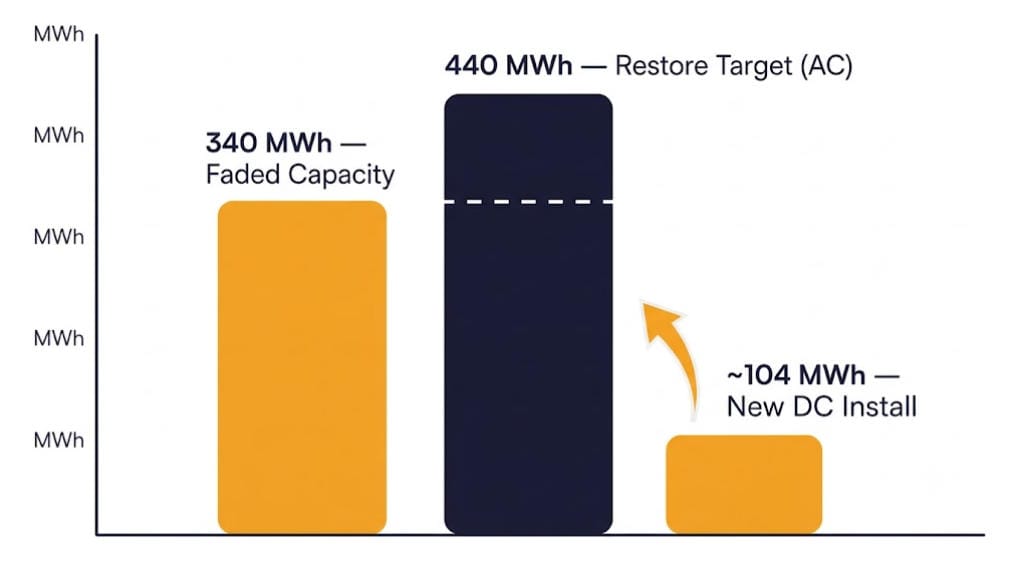
Sizing starts at the point of interconnection, not at the battery rack. Consider a 100 MW, 400 MWh project. After five years, it has faded to 340 MWh of usable energy at the AC side. The operator, in this case, wants to restore headroom to 110 percent of nameplate, or 440 MWh.
That means the project needs 100 MWh of additional AC-side energy. Because DC-to-AC conversion is not lossless, the DC installation must be larger than the AC target. At a typical round-trip factor near 96.5 percent, for example, the operator installs about 104 MWh of new DC capacity to deliver 100 MWh at the AC side.
This buffer-based approach, in short, avoids a common trap. Sizing an augmentation exactly to today’s shortfall just guarantees another shortfall, and another expensive site visit, a year or two later.
AC Block Addition vs. DC Shuffling: At a Glance
| Dimension | AC Block Addition | DC Shuffling |
| New grid connection required | Usually, yes | Usually, no |
| Typical capital cost | Higher | Lower |
| Footprint | Larger — new PCS, transformer, switchgear | Smaller — reuses existing enclosures |
| Chemistry flexibility | Any chemistry | Must match voltage/SOC with existing cells |
| PCS / protection impact | New PCS; new fault-current source to coordinate | Existing PCS; busbar and breaker ratings cap headroom |
| Typical permitting timeline | Months — new interconnection study | Weeks to months — often no new grid approval |
| Best fit | Later-life projects, chemistry upgrades, PCS refresh | Earlier-life projects with headroom in the existing bus |
Choosing Between AC Block Addition and DC Shuffling
When AC Block Addition Makes Sense
AC block addition tends to make sense later in a project’s life, once the original PCS is also due for a technology refresh. It is also the better fit when an operator wants to introduce a different battery chemistry, such as pairing a sodium-ion block with an existing LFP fleet.
When DC Shuffling Makes Sense
DC shuffling, on the other hand, fits best earlier in a project’s life, while the existing busbar and breakers still have headroom. It also suits sites where a new interconnection study would be slow or costly. As cell sizes grow past 500 Ah and system voltages rise, some integrators expect DC block designs, and DC shuffling along with them, to look different in the next generation of projects.
Key Takeaways: AC Block Addition vs. DC Shuffling
1. Degradation is inevitable — plan for it before contracted capacity is at risk.
2. Restore buffers are set in AC terms at the point of interconnection, but installed as DC energy.
3. AC block addition costs more but sidesteps chemistry-matching and synchronization limits.
4. DC shuffling costs less but is capped by busbar, breaker, and voltage-matching limits.
5. The right path depends on project age, available headroom, and permitting timeline.
FAQ About AC Block Addition and DC Shuffling
What Is AC Block Addition?
AC block addition is one way to carry out BESS augmentation. It installs a new, independent power block, complete with its own inverters, next to an existing system, to restore or increase capacity lost to degradation.
Does DC Shuffling Alone Add Capacity?
No. Shuffling alone just reorganizes existing modules for better balance. Capacity, however, is only added when new racks get installed behind the shuffled system.
How Much Does This Augmentation Path Cost?
Cost varies by project size, chemistry, and the path chosen. DC shuffling generally costs less per MWh added, since it reuses the existing PCS and transformer. AC block addition, by contrast, costs more, but it includes new power conversion equipment.
Does DC Shuffling Require New Interconnection Permits?
Usually not. Since no new physical connection is made to the grid, DC shuffling can often bypass a fresh interconnection study. AC block addition, on the other hand, usually cannot.
Can AC Block Addition Mix Battery Chemistries?
Yes. Because the new block has its own PCS and DC bus, it does not need to match the voltage or chemistry of the existing system.
Further Reading
- BESS Augmentation: The Complete Guide
- Mixed-Age String Design After BESS Augmentation
- BESS PCS Functions and Features
- Grid-Forming vs. Grid-Following BESS
- BESS Short Circuit Protection
- PCS Overvoltage Protection
- Understanding BESS Specifications
- AC and DC Augmentation in BESS — Energy-Storage.News
- Augmentation: What Is It and Why Is It Important to BESS? — Modo Energy
BESS Augmentation: The Complete Guide to Restoring Capacity Lost to Degradation
BESS augmentation is the process of adding new battery capacity to an existing energy storage system. It restores or increases capacity lost to degradation. Every BESS loses usable capacity over time. Cycling wears down the cells. Calendar aging adds to it too, even when the system sits idle. So, eventually, the project can no longer deliver the energy or power it promised. BESS augmentation exists to close that gap. It does this by restoring nameplate capacity, or by pushing past it.
| Quick Answer BESS augmentation adds new battery capacity to an existing system, later in its life, to restore or increase capacity lost to degradation. It differs from oversizing, which installs extra capacity upfront. Owners execute augmentation one of two ways: AC block addition, which adds a new self-contained power block, or DC shuffling, which reallocates and adds capacity behind the existing inverters. |
What Is BESS Augmentation?
BESS augmentation and BESS oversizing solve the same problem. However, they act at different points in a project’s life. Oversizing installs extra capacity on day one. This happens before any degradation occurs. BESS augmentation, on the other hand, adds capacity later. It happens once real-world fade has been measured. Our BESS oversizing guide covers that upfront strategy in full. It also covers the trade-off between the two paths. This guide, instead, focuses on the mid-life path. It covers what triggers augmentation, how it works, and how to plan for it.
BESS Augmentation vs. Oversizing: The Short Version
Neither strategy is strictly better. Oversizing locks in capital and tax credits early. But it carries idle capacity for years. BESS augmentation, in contrast, defers that capital. It depends on good execution years later. By then, battery prices, chemistry options, and site conditions may all have changed.
| Factor | BESS Augmentation (Mid-Life) | BESS Oversizing (Upfront) |
| Capex timing | Deferred to year 5-10 | Higher Day-1 cost |
| Section 48E ITC eligibility | Can face reduced eligibility on added capacity | Full credit on entire capacity at commissioning |
| Execution risk | Depends on future prices, chemistry, site conditions | Locked in at commissioning |
| Physical planning | Needs reserved space and headroom | Full footprint installed upfront |
| Best fit | Falling-price markets, budget-constrained projects | ITC-sensitive, stable-forecast projects |
Why Projects Need BESS Augmentation
Lithium-ion cells fade with every charge and discharge cycle. Specifically, the protective layer on the anode cracks and reforms with each cycle. This consumes active lithium. High charge rates and cold temperatures also speed up the damage. Meanwhile, calendar time adds a slower fade on top of cycling.
For some grid-scale LFP projects, usable-capacity fade may average around 2–3% per year, but actual degradation varies substantially with operating conditions, climate, duty cycle, and cell design. As a result, after five to seven years, many projects fall short of their contracted energy or power. That, in turn, threatens revenue directly.
Capacity Guarantees and Tolling Agreements
Most utility-scale BESS projects operate under a tolling agreement or a capacity sale agreement. These contracts are priced against a guaranteed deliverable capacity. This is not simply nameplate capacity at commissioning. So, if degradation erodes that capacity below the contracted floor, trouble follows. The owner then faces liquidated damages or lost revenue. BESS augmentation, therefore, is how owners keep that promise as the asset ages.
These agreements often run 10 to 20 years. So, the augmentation plan is not an afterthought. Instead, it gets built into the financial model at financial close. It sits alongside the degradation curve and the warranty terms.
The Two Paths to BESS Augmentation: AC and DC
There are two ways to physically carry out BESS augmentation. One works on the AC side. The other works on the DC side.
AC Block Addition
First, AC block addition installs a new, self-contained power block next to the existing system. It comes with its own inverters, and often its own transformer too. Because it does not share a DC bus with the old batteries, it avoids voltage and state-of-charge mismatches. It also works with any battery chemistry. As a result, it opens the door to pairing a newer chemistry with an aging LFP fleet.
DC Shuffling
Second, DC shuffling reorganizes existing battery modules behind the inverters already on site. It does not add capacity by itself; additional capacity requires installing new battery modules or racks. It reuses the existing power conversion equipment. This, in turn, keeps costs down. However, busbar ratings, breaker capacity, and voltage matching all place a ceiling on how much it can add.
When new and aged modules share the same DC string, however, the design becomes more complex. For the BMS and string-level considerations, see our guide to Mixed-Age String Design After BESS Augmentation.
For a detailed technical comparison of these two approaches, see our guide to AC block addition vs. DC shuffling guide walks through the full technical comparison. It includes a worked example for sizing the restore buffer. It also covers the busbar and short-circuit limits that cap DC shuffling.
What Triggers a BESS Augmentation Decision?
BESS augmentation planning typically starts at a trigger point. That point is when a site’s measured state of health nears the level needed for its contracted output. Operators track this through periodic capacity tests. In addition, battery management system state-of-health estimates support the tracking. So, neither relies on guesswork.
Typical Timing: Year Five to Year Ten
For most grid-scale LFP projects, that point arrives between year five and year ten. Cycling intensity and climate both affect the timing. For instance, hot climates and aggressive cycling schedules push the timeline sooner. On the other hand, shallow cycling, or oversizing at commissioning, pushes it further out.
Planning early matters a great deal. A reactive BESS augmentation project, ordered only after a shortfall occurs, has far less room to negotiate. Because of that, procurement timelines, chemistry options, and price all suffer.
Battery Chemistry and BESS Augmentation Planning
Battery chemistry affects how easily new capacity can be added. LFP has a relatively flat voltage curve, which can make voltage matching less restrictive than with chemistries such as NMC. However, old and new LFP modules still require careful matching of SOC, SOH, resistance, voltage limits, and BMS behavior before they are combined. This is one reason DC shuffling is more common on LFP systems.
AC block addition, however, removes chemistry matching from the equation entirely. The new block runs its own inverters. So, an operator can add a different chemistry, such as sodium-ion, next to an existing LFP fleet. No voltage curves need to line up.
Tax Credits, Costs, and Procurement for BESS Augmentation
The tax picture for BESS augmentation is less favorable than for oversizing. Under Section 48E, the tax credit applies most cleanly to capacity installed at commissioning. The tax treatment of capacity added through mid-life augmentation can differ from capacity installed at initial commissioning. Project owners should confirm current Section 48E eligibility and applicable requirements with qualified tax advisors before making the augmentation decision. It can also add compliance work. This is a core trade-off against upfront oversizing. So, model it carefully before committing to a mid-life augmentation strategy.
Procurement timelines also differ sharply between the two paths. DC shuffling makes no new grid connection. So, it can often skip a fresh interconnection study. AC block addition, in contrast, usually cannot skip that step, since it adds new grid-connected hardware. That difference alone can add months to the schedule.
Cost varies too. DC shuffling generally costs less per megawatt-hour added. This is because it reuses the existing PCS, transformer, and switchgear. AC block addition costs more. However, it buys a clean equipment boundary. It also adds the option to upgrade power conversion technology at the same time.
A Practical BESS Augmentation Planning Checklist
1. Confirm the site’s actual state-of-health trend against the contracted capacity floor.
2. Model the restore buffer in AC terms, then convert it to a DC installation size, accounting for round-trip losses.
3. Choose between AC block addition and DC shuffling based on busbar/breaker headroom, chemistry needs, and permitting timeline.
4. Reserve physical space for future modules if a DC shuffling path is likely.
5. Model the Section 48E tax credit and financing impact of adding capacity mid-life.
6. Build procurement and, if needed, interconnection lead time into the schedule early.
Key Takeaways on BESS Augmentation
1. BESS augmentation restores or increases capacity lost to degradation, later in a project’s life.
2. Most grid-scale LFP projects need to plan for it between year five and year ten.
3. Tolling agreements and capacity sale agreements make augmentation a contractual necessity, not an option.
4. AC block addition and DC shuffling are the two execution paths, with different cost, timeline, and chemistry trade-offs.
5. Augmented capacity can face reduced Section 48E tax credit eligibility compared to capacity installed at commissioning.
Frequently Asked Questions About BESS Augmentation
When Should a Project Plan for BESS Augmentation?
In short, BESS augmentation planning should begin early. It should start as soon as a site’s degradation curve first threatens a future contract obligation. It should not wait until after a shortfall occurs.
What’s the Difference Between BESS Augmentation and BESS Oversizing?
Oversizing installs extra capacity upfront, before degradation happens. BESS augmentation, by contrast, adds capacity later, once real-world fade has been measured. Oversizing generally captures a fuller tax credit. It also carries lower operational complexity. Augmentation, however, defers capital and can benefit from falling battery prices.
Does Augmented Capacity Qualify for the Section 48E Tax Credit?
Capacity installed at commissioning generally qualifies most cleanly for the Section 48E credit. Capacity added later through augmentation, however, can face reduced eligibility or added compliance work. So, this should be modeled carefully before choosing a mid-life strategy.
How Long Does a BESS Augmentation Project Take?
Timelines vary by path. DC shuffling projects typically avoid a new interconnection study. So, they can often move in weeks to a few months. AC block addition projects, on the other hand, usually require new grid-connected hardware. As a result, they more commonly take several months, due to interconnection and permitting steps.
What’s the Difference Between AC Block Addition and DC Shuffling?
AC block addition installs a new, independent power block with its own inverters. It works with any battery chemistry. DC shuffling, in contrast, reallocates and adds capacity behind the existing inverters. It costs less, but it is limited by busbar, breaker, and voltage-matching constraints.
Further Reading
- BESS Oversizing: Pros, Cons & the Right-Sizing Strategy
- AC Block Addition vs. DC Shuffling
- Mixed-Age String Design: Managing a BESS String After Augmentation Adds New Cells
- Understanding BESS Specifications
- Battery State of Health (SoH) Estimation Guide
- What Is a Tolling Agreement in BESS? — BESS.courses
- Augmentation: What Is It and Why Is It Important to BESS? — Modo Energy
PCS Overvoltage Protection: Coordinating Transformer and Inverter Defense Against High-Voltage Grid Faults
Key Takeaway
PCS overvoltage protection is the layered set of defenses that keeps power conversion systems and transformers online, and undamaged, when grid voltage swells past normal limits. It combines fast surge arresters, DC-bus crowbar circuits, software ride-through control, and coordinated relay settings into one system. So it does not treat the transformer and the inverter as separate problems.
In short, it lines up transformer insulation limits with inverter chip limits. When a high-voltage grid fault hits, ride-through control briefly adjusts reactive current. At the same time, surge arresters and firmware limits shield the delicate IGBT or SiC switches from damaging voltage spikes.
Modern grid codes such as IEEE 1547-2018 require both to stay connected through many of these events. As a result, protection has to work in layers. It also has to be planned jointly. Get the coordination wrong, and the surge arrester clamps too late. Or, just as often, the PCS rides through longer than the transformer’s insulation can bear.
| Quick Answer PCS overvoltage protection combines transformer-side relays (ANSI 59, ANSI 24), surge arresters, and differential protection (ANSI 87T) with PCS-side defenses (DC-bus crowbar circuits, ride-through control, gate-driver clamps). The two systems must be coordinated. Specifically, the arrester should clamp below the PCS trip threshold. Also, the ride-through duration should stay inside the transformer’s short-time withstand rating, per IEEE C57.12. |
Why PCS Overvoltage Protection Differs From Overcurrent Protection
Most protection engineers think in terms of overcurrent first. So fuses, breakers, and relays are usually sized to clear a fault before wires or windings overheat. Voltage swells flip that logic around. Here, the equipment is not drawing too much current. Instead, it is facing too much voltage. So the failure paths are different:
- Load rejection — a large downstream load trips offline, and voltage spikes upstream before regulation catches up
- Single-line-to-ground faults on ungrounded or high-impedance grounded systems, which can push healthy phases toward line-to-line voltage
- Switching transients from capacitor bank energization, transformer tap changes, or line reclosing
- Ferroresonance, more common on lightly loaded systems with long cable runs
Overall, the transformer and the PCS each feel this stress in their own way. That is why PCS overvoltage protection needs two coordinated strategies, not one shared setting. For reference, full ride-through requirements sit inside IEEE 1547-2018, the standard most U.S. interconnection agreements now reference.
Transformer-Side Defenses That Support PCS Overvoltage Protection
Insulation and Core Stress From Sustained Overvoltage
Sustained overvoltage raises the transformer’s flux density. This pushes the core toward saturation. As a result, a saturating core draws jagged, inrush-like current. It also creates hot spots in the windings. Over time, the added vibration and noise speed up insulation aging.
In short, the standard protection layers are:
- ANSI 59 (overvoltage relay) — inverse-time or definite-time curves set to match the interconnection standard’s HVRT voltage-duration envelope
- ANSI 24 (volts/hertz protection) — catches overexcitation specifically. A plain overvoltage relay does not track the frequency side of core saturation. So this is a separate layer, not a substitute
- Surge arresters (gapped silicon-carbide or MOV-based) on both HV and LV terminals, sized to the transformer’s Basic Insulation Level (BIL)
Dielectric Stress From Fast Transients
Switching surges hit inter-turn winding insulation on a fast timescale. Relays cannot catch it. Specifically, that timescale runs sub-millisecond. Protective relaying, by contrast, works over cycles to seconds. So surge arresters and terminal snubber circuits carry the real burden here. By the time an ANSI 59 or 24 element reacts, the fast transient is already gone.
Differential and Overcurrent Protection (ANSI 87T, 50/51)
Alongside overvoltage-specific relaying, transformer protection schemes standardly add two more layers.
Differential protection (ANSI 87T) compares current entering the HV side against current leaving the LV side. It uses Kirchhoff’s Current Law to do this. A mismatch past a set threshold signals an internal winding fault. It trips the breaker within roughly 30 ms. However, inrush and magnetizing current during energization or overvoltage can also create a differential current. So modern relays use harmonic restraint. This tells real faults apart from these normal transients.
Overcurrent and earth fault protection (ANSI 50/51) clears sustained high fault current from grid-side short circuits. It uses instantaneous (50) and inverse-time (51) elements. These typically sit behind the differential scheme. Instead, they act as backup protection, not the first line of defense. Engineers also selectively coordinate the trip settings, so the device closest to a fault clears it first and leaves the rest of the system energized.
Voltage Regulation via On-Load Tap Changers (OLTC)
A BESS often connects to a weak or highly variable grid. There, an on-load tap changer adjusts the transformer’s turns ratio while it stays in service. This holds secondary-side voltage within range without shutting the unit down. So OLTCs offer a slower, mechanical form of voltage regulation. They help absorb sustained voltage drift from renewable generation. But they cannot replace surge arresters or relay protection against fault-driven transients.
Grounding and Shielding
- Low-impedance grounding grid — the transformer enclosure, surge arresters, and PCS frame should bond to the same grounding network. This limits ground potential rise during a fault. It also keeps protective devices on a common reference.
- Electrostatic shielding — an interwinding shield between primary and secondary cuts high-frequency noise and voltage-spike coupling from the grid side into the PCS side. It works alongside surge arrester protection, not in place of it.
PCS Overvoltage Protection: Inverter-Side Defenses
The inverter’s semiconductor switches, whether IGBT or SiC, face DC-bus overvoltage that flows back from an AC-side voltage swell. That exposure gets worse during unbalanced faults. There, the control loop’s own feedback signal becomes thrown off.
DC-Bus Overvoltage Protection
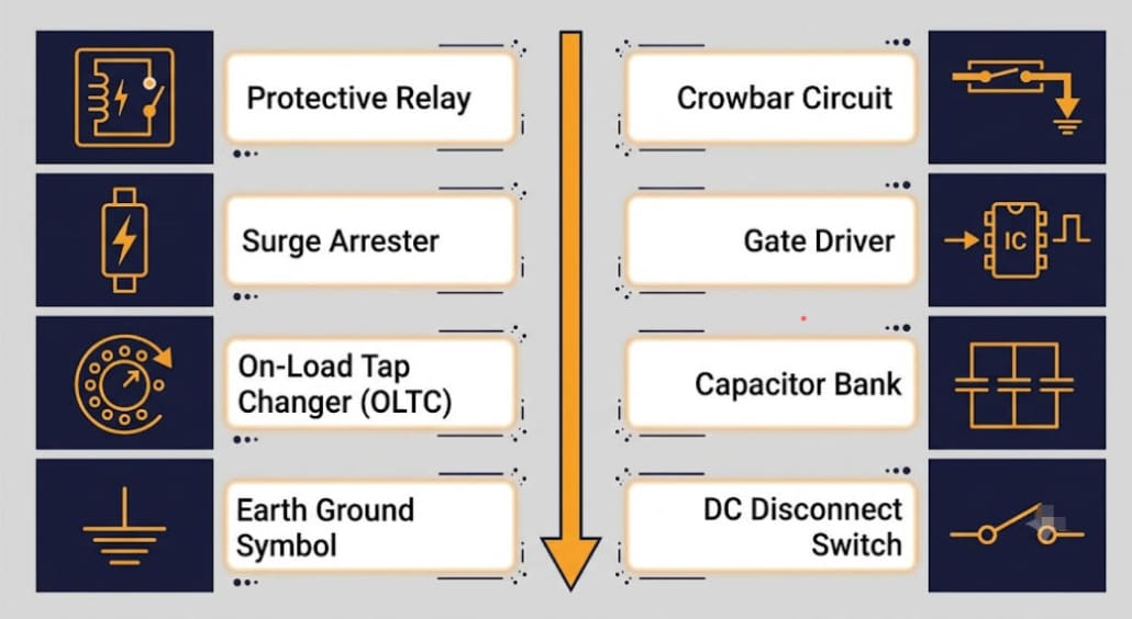
Braking choppers or crowbar circuits dump excess energy into resistors once bus voltage crosses a threshold. This protects the DC-link capacitors and the switches from overvoltage. Usually, it is the first active layer of PCS overvoltage protection to engage during a swell. DC contactors, meanwhile, serve as a hardware failsafe. They isolate the battery racks if the chopper alone cannot keep bus voltage inside a safe window.
AC Overvoltage Ride-Through Control
Older firmware tripped the PCS offline at the first sign of a swell. Modern firmware, built to current interconnection standards, keeps the PCS connected instead. Under IEEE 1547-2018’s default Category III envelope, for example, the PCS must ride through up to 1.10 per-unit for 2 seconds. Between 1.10 and 1.20 per-unit, it can briefly cease energizing instead of disconnecting outright. Above 1.20 per-unit, a full trip is required.
Also, the PCS actively absorbs reactive power, or VARs, to help pull grid voltage back down. As a result, the PCS becomes part of the fix, not just a bystander that disconnects. The LVRT and HVRT ride-through curves that govern this behavior work the same way in both directions. They are just mirrored for sags versus swells.
Volt-VAR and Volt-Watt Curve Control
Ride-through handles transient swells. But IEEE 1547-2018 also standardizes a separate, ongoing grid-support function for milder, sustained overvoltage. When a utility activates it, the PCS runs a volt-VAR curve. Below 1.02 per-unit voltage, the curve sits in a dead zone, and the PCS adds no reactive power. Above that, it starts absorbing reactive power, reaching its full absorption limit at 1.08 per-unit. These are the default curve settings described in a recent IEEE-affiliated study.
Some interconnection agreements also activate volt-watt control. This trims active power output if voltage stays high despite the reactive response alone. It works alongside volt-VAR, not in place of it.
Negative-Sequence Current Limiting
Unbalanced high-voltage faults produce negative-sequence currents. These heat phase legs unevenly. So control loops need an explicit limit here, separate from the general overcurrent limit. Otherwise, a single-phase-biased fault could overheat one leg while the others stay fine.
Fast Semiconductor-Level PCS Overvoltage Protection
Gate-driver desaturation detection and hardware-level overvoltage clamps work in microseconds. They act independently of the software control loop, and faster than it. As a result, they serve as the last line of defense when everything upstream fails to act in time.
Anti-Islanding and Ride-Through Coordination
A high-voltage fault can sometimes cascade into a full outage. When that happens, the PCS must detect that it is energizing a dead section of grid, then disconnect. IEEE 1547-2018 requires this within 2 seconds of island formation. Detection methods split into two types. Passive methods watch for abnormal voltage, frequency, or phase jumps. Active methods, instead, inject a small perturbation, such as a frequency drift, to force a detectable response if the grid is truly gone.
There is a real design tension here. Specifically, a 2019 NREL laboratory study found that ride-through behavior can noticeably slow islanding detection. Even so, run-on times stayed inside the 2-second IEEE 1547-2018 window in every case tested. That happens because a PCS holding voltage and frequency steady during a disturbance can look like a healthy grid connection. For this reason, ride-through and anti-islanding logic need coordinated tuning. They should not run as independent settings. For the full technical report behind this finding, see the Sandia National Laboratories study on OSTI.
Active Voltage Conditioning
Some sites see voltage that never settles, beyond what ride-through settings alone can absorb. For these sites, dedicated power-electronic conditioners sit in-line ahead of the main PCS. One example is ABB’s PCS100 AVC-40, rated from 225 kVA to 3,600 kVA with efficiency above 98 percent.
These units fix sags and swells within milliseconds. Even so, this is an extra device for grids that are weak or noisy all the time. It cannot replace the PCS’s own ride-through and protection functions.
Comparison: Transformer vs. PCS Overvoltage Protection
Overall, the table below lines up each side’s defenses by timescale. This makes the gaps between them easy to spot at a glance.
| Protection layer | Transformer | PCS |
|---|---|---|
| Primary threat | Core saturation, insulation aging | DC-bus overvoltage, switch stress |
| Slow protection (cycles–seconds) | ANSI 59 / ANSI 24 relays, ANSI 50/51 overcurrent | Software-based AC overvoltage ride-through control |
| Internal fault detection | ANSI 87T differential protection | Negative-sequence current limiting |
| Fast protection (µs–ms) | Surge arresters, terminal snubbers | Gate-driver desaturation, hardware clamps |
| Energy dissipation | Arrester let-through to ground | Braking chopper / crowbar resistors |
| Sustained voltage drift | On-load tap changer (OLTC) | Active voltage conditioning (external, supplementary) |
| Outage/dead-grid response | Coordinated with PCS anti-islanding | Anti-islanding, disconnect within 2s (IEEE 1547-2018) |
| Fault type most sensitive to | Single-line-to-ground on ungrounded systems | Unbalanced faults (negative-sequence) |
| Governing standard | IEEE C57.12 series | IEEE 1547-2018, UL 1741 SB |
Coordinating Transformer and PCS Overvoltage Protection
Treating these as two independent systems is a common design gap. So three coordination checks matter most for site-wide PCS overvoltage protection.
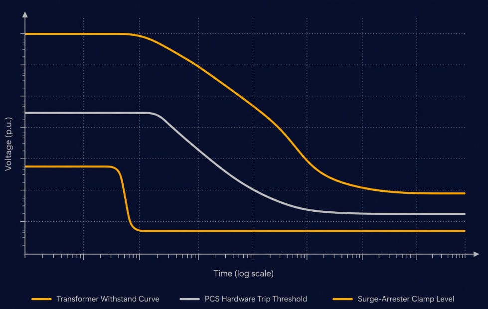
- Let-through voltage vs. PCS trip threshold. The transformer’s surge arrester should clamp transients below the PCS’s hardware overvoltage trip point. This way, the arrester absorbs the transient, not the PCS’s own protection.
- HVRT duration vs. transformer withstand. The voltage-time ride-through curve set in the PCS needs to sit inside the transformer’s short-time overvoltage withstand rating, per IEEE C57.12. Otherwise, the PCS could ride through an event longer than the transformer can structurally take.
- Grounding configuration vs. overvoltage settings. How the system is grounded — solidly grounded, resistance-grounded, or ungrounded — directly sets how much overvoltage a single-line-to-ground fault produces on the healthy phases. This needs joint modeling with the PCS overvoltage settings during system design. It should not be a decision each discipline makes on its own.
- Selective tripping. Transformer relay settings and the PCS’s own protection should be time-graded, so a fault on the PCS side clears at the device closest to it first. Otherwise, a local fault trips more of the system than it needs to.
- Fault current contribution vs. inverter control mode. The differential (87T) and overcurrent (50/51) settings assume a certain fault current magnitude to detect against. A grid-following PCS contributes only limited fault current during a fault, while a grid-forming PCS contributes significantly more. So these relay settings should be checked against which control mode the PCS actually runs — see our grid-forming vs. grid-following BESS guide for the underlying comparison.
Governing Standards for PCS Overvoltage Protection
- IEEE 1547-2018 — interconnection requirements for distributed energy resources, including HVRT voltage-duration curves
- UL 1741 SB — certification testing that verifies HVRT compliance for grid-support equipment
- IEC 61000-4-11 / IEC 61000-4-34 — voltage dip and swell immunity testing for equipment rated below and above 16 A per phase
- IEEE C57.12 series — transformer design and short-time overvoltage withstand standards
For system designers weighing broader grid-support tradeoffs, this same coordination logic also shows up in Fast Frequency Response design. There, too, BESS control settings must stay inside both a grid-code window and the hardware’s own physical limits.
Key Takeaways for PCS Overvoltage Protection Design
| Point | Why It Matters |
|---|---|
| Voltage swells stress equipment differently than overcurrent faults | Insulation and semiconductor limits, not wire heating, drive the failure modes |
| Transformer and PCS need separate, coordinated protection layers | A single shared setting misses the different timescales each device needs |
| Surge arresters and relays cover different timescales | Arresters catch microsecond transients; relays catch cycles-to-seconds events |
| Ride-through duration must stay inside transformer withstand ratings | Otherwise the PCS can hold an overvoltage longer than the transformer can survive |
| Anti-islanding and ride-through logic must be tuned together | Ride-through behavior can otherwise slow dead-grid detection |
FAQ
What’s the Difference Between LVRT and HVRT?
LVRT, or Low Voltage Ride-Through, keeps equipment connected during voltage sags. These are typically caused by faults or heavy load switching. HVRT, or High Voltage Ride-Through, does the same for voltage swells instead. So the control challenges largely mirror each other. But the hardware failure modes differ. Sags stress current limits. Swells stress insulation and semiconductor overvoltage limits instead. For the underlying voltage-duration curves, see our full LVRT and HVRT guide.
Why Does the PCS Absorb Reactive Power During a High-Voltage Fault Instead of Just Disconnecting?
Modern grid codes require ride-through for a clear reason. Mass disconnection of distributed generation during a voltage event can worsen grid instability. So absorbing VARs actively helps pull the voltage back toward normal. As a result, the PCS becomes part of the grid’s self-correction, not a source of added disturbance. For more on how this reactive-power capability is sized and rated, see our BESS power factor guide.
Can a Surge Arrester Alone Provide PCS Overvoltage Protection?
No. Arresters handle fast transients, such as switching surges and lightning-induced events. They work on a timescale of microseconds to milliseconds. Sustained overvoltage from load rejection or a ground fault lasts cycles to seconds instead. That needs the PCS’s own ride-through control. Where ride-through limits run out, it also needs overvoltage relay protection. In short, the two protection types are not interchangeable.
Does Ride-Through Conflict With Anti-Islanding Requirements?
They can pull against each other. Anti-islanding must detect a dead grid and disconnect within 2 seconds under IEEE 1547-2018. Ride-through, meanwhile, is built to keep the PCS connected through a disturbance rather than tripping. A 2019 NREL study found ride-through can slow islanding detection. That happens because a PCS holding voltage and frequency steady during the event looks like a stable grid connection. For this reason, both functions need tuning together at commissioning. Neither should be set on its own.
Why Must PCS Overvoltage Protection Settings Match the Transformer’s Withstand Rating?
Say the PCS’s HVRT setting runs longer than the transformer can withstand. The PCS still stays connected and rides through the event as designed. But the transformer can suffer accelerated insulation aging. In a severe enough event, it can suffer immediate insulation failure instead. That happens because it sits at an overvoltage level longer than its short-time withstand rating allows. This is the core reason the two systems’ settings need coordination at the design stage. They should not be configured apart from each other.
Further Reading
LVRT and HVRT: Voltage Ride-Through for BESS and Solar
Fast Frequency Response (FFR): How BESS Stabilizes Grid Frequency in Milliseconds
BESS Short Circuit Protection: A Layered Approach to Preventing Fires in Grid-Scale Battery Storage
Grid-scale batteries rarely fail from one single problem. A small fault grows step by step until it becomes a fire — that is the real story behind BESS short circuit protection.
It is not one part. It is not one sensor.
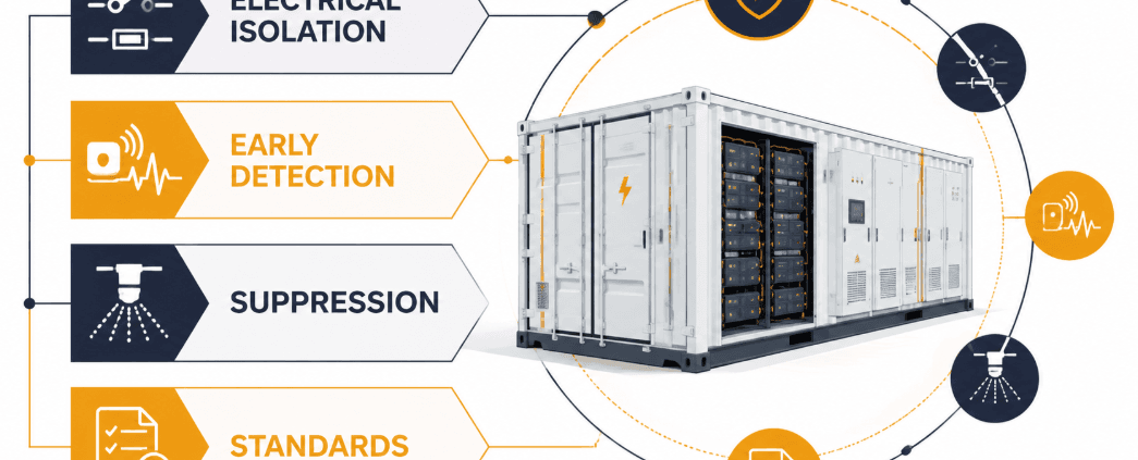
Good BESS short circuit protection is four layers working together: electrical isolation, early detection, suppression, and design standards. Miss one layer, and the rest have to work much harder to catch the fault in time.
For more on how the power conversion system contributes to fault behavior, see our guide on BESS PCS functions and features.
Quick Answer: What Is BESS Short Circuit Protection?
| Quick Answer BESS short circuit protection combines four layers. First, fast electrical isolation (fuses, contactors, gate drivers) stops a fault at the source.Second, early detection (off-gas sensors, thermal imaging, cell-level BMS) catches trouble minutes before flames appear.Third, suppression systems (venting, clean-agent, water-mist) contain what detection could not prevent.Fourth, design standards (NFPA 855, UL 9540/9540A) govern how the first three layers get specified, tested, and installed. |
Key Takeaways
| Layer | What It Does | Example Components |
|---|---|---|
| Electrical isolation | Stops the fault before it makes enough heat to ignite anything | Fuses, rack disconnects, IGBT gate drivers, propagation barriers |
| Early detection | Flags a developing problem minutes before ignition | Off-gas sensors, thermal cameras, cell-level BMS |
| Suppression | Contains what detection could not prevent | Deflagration vents, clean-agent systems, water-mist |
| Standards | Governs how every other layer is tested and installed | NFPA 855, UL 9540, UL 9540A |
Why “Short Circuit” Isn’t the Whole Story in BESS Short Circuit Protection
Most large battery fires get called short-circuit fires. But that label is a bit misleading.
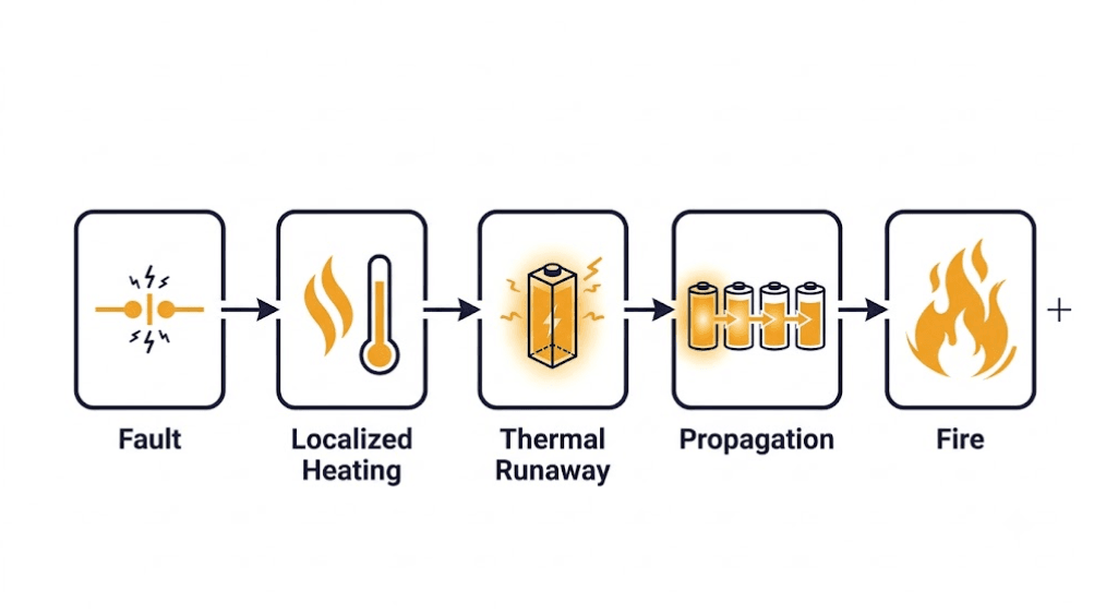
What actually happens is thermal runaway that spreads from cell to cell, like dominoes falling.
A short circuit is often the trigger, whether it comes from an internal cell defect, an external fault, or a loose connection.
Still, the real danger comes later, once heat from that one cell starts moving outward. Good BESS short circuit protection has to account for both stages, not just the initial fault.
This distinction shapes how each protective layer gets designed. For example, off-gas detection is not really a short-circuit sensor.
It is a thermal-runaway precursor sensor instead. It picks up gases vented during early cell decomposition.
Often, this happens before a short circuit or flame shows up on any other instrument.
Once you see the full chain — fault, then localized heating, then thermal runaway, then propagation, then fire — it becomes clear where each layer of BESS short circuit protection actually steps in.
Layer 1: Electrical Isolation for BESS Short Circuit Protection
The first job of electrical isolation is simple: keep a fault from ever reaching the point of ignition.
Fast-Acting Fuses and Rack-Level Disconnects
High-speed fuses at the string and pack level interrupt overcurrent fast. They act before it builds up enough localized heat to start thermal runaway.
Also, many newer systems add rack-level contactors and disconnects. As a result, a single faulted rack can be isolated without shutting down the whole container.
This cuts both fire risk and downtime at the same time.
IGBT Protection and Physical Separation
Active gate drivers watch the IGBTs (insulated-gate bipolar transistors) in the power conversion system. If overcurrent shows up, they shut the IGBTs down fast and safely.
This protects both the PCS and the battery side of the connection.
Keeping power conversion gear apart from the battery blocks matters too. A PCS-side fault tends to carry more energy, so keeping it separate makes it less likely to ignite the battery enclosure.
Cell-to-Cell Propagation Barriers
Thermally insulating materials sit between cells and modules. Mica sheets, aerogel layers, and phase-change barriers are common choices.
Even so, if one cell enters thermal runaway, these barriers slow the heat transfer. That extra time often lets detection and suppression systems do their job.
Layer 2: Early Detection Catches the Fault Before It Spreads
A detection layer only matters if it catches trouble minutes, not seconds, before ignition. This is where BESS short circuit protection depends most on speed.
Off-Gas Detection
Specialized sensors pick up gases released during early battery decomposition. Carbon monoxide, hydrogen, and various volatile organic compounds are the usual signs.
Often, this happens minutes before any smoke or measurable temperature rise. So most safety engineers treat off-gas detection as the earliest reliable warning inside a BESS enclosure.
Thermal Imaging and Smart BMS
Continuous infrared monitoring flags hot spots on busbars, connections, and power electronics. These are common origin points for electrical faults.
At the same time, a smart Battery Management System watches voltage and temperature at the individual cell level. It does not stop at the module or rack level.
That granularity lets a developing imbalance get caught and isolated before it touches neighboring cells.
Layer 3: Fire Suppression Contains What Detection Could Not Prevent
Even strong prevention and detection will not stop every event. Suppression systems act as the last line of defense.
Also, code increasingly treats them as mandatory rather than optional.
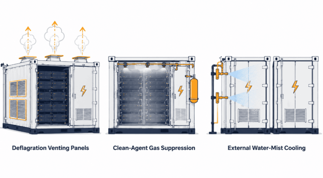
Deflagration Venting
Explosion venting panels direct overpressure from vented battery gases safely upward. This keeps pressure away from people and nearby equipment.
As a result, pressure cannot build up inside the enclosure in the first place.
Clean-Agent Suppression Within BESS Short Circuit Protection
Clean-agent systems flood the compartment and interrupt the fire’s chemical reaction. Unlike sprinklers, they avoid water damage and electrical risk.
But not all agents work the same way. Novec 1230 is a clean gaseous agent that displaces oxygen and absorbs heat.
Stat-X, on the other hand, is a condensed aerosol that suppresses fire through a different chemical mechanism.
So the right choice depends on compartment size, ventilation design, and re-entry time requirements.
Water-Mist and Deluge Cooling
External water-mist or deluge systems usually do not stop the fire that started the event. Instead, their job is cooling adjacent containers.
This keeps the fire from jumping to the next unit. Since container-to-container spread is where the largest-scale incidents tend to originate, cooling matters as much as suppression.
| Suppression Type | Primary Function | Best Suited For |
|---|---|---|
| Deflagration venting panels | Relieve gas overpressure safely | Preventing explosion or enclosure rupture |
| Clean-agent (Novec 1230, Stat-X) | Interrupt fire chemistry, no residue | In-compartment suppression, electronics-safe |
| Water-mist / deluge | External cooling | Preventing container-to-container propagation |
Layer 4: NFPA 855 and UL 9540A Set the Rules for BESS Short Circuit Protection
Each safety part only works as a system if it follows a recognized standard. That is where NFPA 855 and UL 9540/UL 9540A come in for BESS short circuit protection.
What NFPA 855 Covers
NFPA 855 covers siting, spacing, detection, and suppression. It also covers ventilation and emergency response planning.
One common example is the minimum 3-foot (914 mm) gap required between ESS units. This can shrink if large-scale fire testing shows a closer gap is safe.
Also, the 2023 edition made fire suppression mandatory for nearly all ESS installations.
The 2026 edition goes further still. It expands formal Hazard Mitigation Analysis to most BESS sites, not just large ones.
For the full breakdown of scope, thresholds, and the 2026 changes, see our NFPA 855 guide.
UL 9540 vs. UL 9540A in BESS Short Circuit Protection
These two standards sound alike but do different jobs. UL 9540 is a system-level product certification.
A large-scale fire test method, UL 9540A generates the propagation data regulators use to set spacing, suppression, and ventilation rules under NFPA 855. It is not a certification by itself.
For the full breakdown of how these two standards interact, and why the distinction affects permitting timelines, see our dedicated guide: UL 9540 vs UL 9540A: Understanding the Key Differences.
Emergency Response Plans
NFPA 855 also requires written emergency plans. These cover safe shutdown steps and coordination with local fire crews.
It is easy to treat this requirement as an afterthought. But it gets flagged often during AHJ review and insurance underwriting.
FAQ: BESS Short Circuit Protection
What is BESS short circuit protection?
BESS short circuit protection combines electrical isolation, early detection, and suppression. Together, they stop a short circuit fault from turning into thermal runaway and fire.
Is a short circuit the same thing as thermal runaway?
No, they are different things. A short circuit is one possible trigger for thermal runaway.
But thermal runaway itself is the underlying cascading failure. So the real fire risk in BESS short circuit protection comes from propagation between cells, not the short circuit event alone.
Is UL 9540A certification required for every BESS project?
Not exactly. UL 9540A is a test method, not a certification. So there is no such thing as being “UL 9540A listed.”
Even so, most commercial and utility-scale projects in the U.S. need UL 9540A test data. Then this data satisfies NFPA 855 and local fire code requirements for permitting.
What is the minimum spacing required between BESS units under NFPA 855?
The commonly cited baseline is 3 feet (914 mm) between individual units.
Even so, this can shrink if large-scale fire testing under UL 9540A documents that a smaller separation is safe for that specific system. Spacing is one of the simplest parts of BESS short circuit protection to verify during a site walk.
Does off-gas detection replace the need for a BMS?
No, the two serve different roles. Off-gas detection is an early warning system inside the enclosure.
It watches for thermal-runaway gases before flames show up.
A cell-level BMS, by contrast, watches voltage and temperature. So it catches a developing fault before it produces measurable off-gas at all. Together, they cover both ends of BESS short circuit protection.
Further Reading
UL 9540 vs UL 9540A: Understanding the Key Differences
UL 9540A Test Method: Complete Guide for BESS Manufacturers
Battery Management System (BMS) Explained
BESS PCS Functions and Features
Fast Frequency Response (FFR): How BESS Stabilizes Grid Frequency
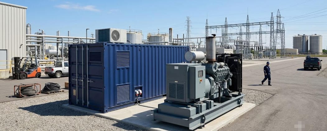
How to Replace a Diesel Generator with BESS: Sizing, Costs, and Case Studies
| Quick answer Diesel generator replacement with BESS works in three steps. First, convert your generator’s kVA rating to real kW using the power factor. Second, size the battery in kWh to your load and backup hours. Third, size the PCS in kW to your peak power, with a margin for inrush. A well-sized system cuts daily fuel cost. It switches in under 20 milliseconds, not 10-30 seconds. Most projects pay back in 4 to 7 years. |
For most commercial and industrial (C&I) sites, diesel generator replacement is not a fringe idea anymore. So it is now a normal line item in capital planning.
Diesel gensets are reliable. But they cost money every hour they run, and they need constant upkeep.
A BESS closes that gap in three ways. First, it starts delivering power in milliseconds. Second, it has no moving parts to wear out. Third, when paired with solar, it can cut fuel use close to zero.
This guide covers the real costs, the sizing math, and the kVA-to-kW conversion your generator needs. Also, it covers PCS choice, four case studies, and a free sizing calculator you can add to this post.
Why Facilities Are Pursuing Diesel Generator Replacement in 2026
Three main pressures are pushing facilities away from diesel power. First, fuel prices remain high and unpredictable. Second, engines with hundreds of moving mechanical parts require constant upkeep. Third, ESG regulations are becoming increasingly strict.
While none of these factors are entirely new, LFP battery costs have dropped significantly in recent years. Consequently, the financial math for generator replacement now works for far more commercial and industrial sites than ever before.
The True Cost of Diesel Generator Replacement
Fuel is the biggest cost of running a generator. Also, it scales with load. For example, a diesel generator burns about 0.07 to 0.08 gallons per kWh at 70-80% load.
A 100 kW generator at 75% load burns about $402 a day in fuel alone. That is about $0.22 per kWh. Also, this does not include oil, filters, or testing costs.
Once labor and parts are added, costs climb further. All-in costs often land between $0.35 and $0.65 per kWh, per 2026 generator operating-cost benchmarking.
Costs climb even more at partial load. In fact, generators run least efficiently below 40% load. That is where most backup units sit most of the time.
Maintenance and Wet-Stacking Problems
Because generators are complex mechanical systems, internal parts like pistons and valves naturally wear down over time. Therefore, they demand regular, costly service intervals.
Additionally, running generators at light loads leads to wet-stacking, which occurs when unburned fuel accumulates inside the exhaust system. As a result, the engine suffers accelerated wear and requires even more maintenance.
In contrast, a BESS has no moving mechanical components; consequently, it requires almost no scheduled maintenance beyond routine inspection checks.
Emissions and ESG Pressure
Because diesel exhaust releases high amounts of NOx, particulate soot, and $\text{CO}_2$, these emissions increasingly trigger warnings on environmental audits and insurance reviews.
However, a BESS creates zero on-site emissions during operation. Furthermore, when paired with a local solar array, overall facility emissions fall close to zero.
Generator kVA, BESS kWh, and PCS kW: Why the Units Are Different
Here is a detail that trips up many buyers. Generators are rated in kVA, not kW. That is apparent power, not real power.
BESS energy is rated in kWh. Also, PCS power is rated in kW. So these three units are not the same.
Mixing them up can badly oversize, or worse, undersize your system. So convert your generator’s rating to real kW first.
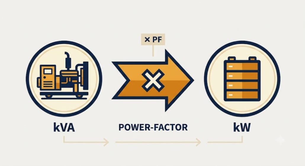
Converting Generator kVA to kW
| kVA to kW Conversion Formula kW = kVA × Power Factor (PF) Industrial loads typically use a default PF of 0.8 unless your generator nameplate or a recent load study states otherwise. |
For example, a 125 kVA generator running at a 0.8 power factor delivers 100 kW of real output (125 x 0.8 = 100 kW). Similarly, a 500 kVA generator at 0.85 power factor yields 425 kW of real power.
Therefore, you must always verify the actual power factor on your generator’s data sheet before sizing your battery system. Otherwise, a single inaccurate assumption will skew all subsequent calculations
Why BESS Uses kWh and PCS Uses kW
A BESS is sized in two distinct steps. First, energy capacity is measured in kWh to determine duration. Second, inverter capacity is measured in kW to handle the load.
Because energy sets runtime while power determines peak instantaneous capacity, confusing these two units often leads to costly site undersizing.
The table below keeps the three units straight.
| Component | Unit | What It Measures |
|---|---|---|
| Diesel generator | kVA (apparent power) | Nameplate rating before power factor is applied |
| Real generator output | kW (real power) | kVA x power factor, the number you actually size around |
| BESS battery | kWh (energy) | How much energy is stored, and how long it can run the load |
| PCS / inverter | kW (power) | How much power it can deliver at any single instant |
Cost Comparison: Diesel Generator Replacement vs. Keeping Your Genset
The table below compares the two options side by side.
| Factor | Diesel Generator | BESS |
|---|---|---|
| Switching time | 10-30 seconds (ATS transfer delay) | Under 20 milliseconds |
| Running cost | $0.22-0.28/kWh fuel at optimal load; $0.35-0.65/kWh all-in | No fuel cost; O&M is largely software-managed |
| Maintenance | Oil, filters, load-bank testing, overhauls | Minimal, no moving parts |
| Emissions | NOx, particulates, CO2 on every run | Zero on-site emissions |
| Fuel logistics | Needs on-site storage and refueling | None |
| Noise | 65-85 dBA typical | Near-silent |
| Typical payback | Not applicable, an ongoing operating cost | 4-7 years via avoided fuel and demand charges |
Most sites do not remove the generator on day one. Instead, they install the BESS first, right alongside the running genset.
The PWRNXT diesel generator replacement program in India uses this same model. So do similar C&I projects elsewhere.
Next, the team tests switching performance on-site. Only then does the generator get downgraded to backup, or retired.
How to Size a BESS for Diesel Generator Replacement
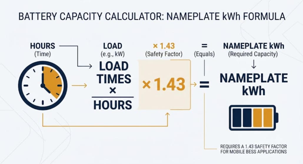
Sizing a BESS depends on two primary metrics: energy (kWh) and power (kW). If you balance this ratio correctly, the system operates seamlessly.
However, if you miscalculate, the battery will either trip under heavy loads or unnecessarily inflate project costs.
Step 1 — Determine Your Critical Load in kW
Pull 12 months of interval data. Or, run a load study during a real outage.
If you only have kVA, convert it to kW first, using the formula above. Then use the load you actually want to keep on.
Full production and critical-circuits-only are very different numbers. So pick the right one upfront.
Step 2 — Determine Required Backup Hours
Base this on real outage history, not a guess. Instead, pull it from utility data or your own outage log.
Weak grids with short, frequent outages need a shorter, high-cycling BESS. Grids with rare but long outages, by contrast, need more stored energy per kW.
Step 3 — Calculate Nameplate Capacity for Diesel Generator Replacement
The baseline formula is shown below.
| BESS sizing formula Usable Energy Required (kWh) = Critical Load (kW) x Backup Duration (hours) Nameplate Capacity (kWh) = Usable Energy Required x 1.2 safety margin / (Depth of Discharge x Round-Trip Efficiency) For LFP at 90% DoD and about 93% round-trip efficiency, this simplifies to: Nameplate Capacity (kWh) = Critical Load (kW) x Backup Duration (hours) x 1.43 |
The 1.2x margin covers load growth and inrush. The DoD and efficiency terms cover two more losses.
First, the energy a lithium battery cannot safely use. Second, conversion losses across the inverter and BMS.
Step 4 — Worked Examples
Here are three quick examples. Each one starts from a real kW figure, already converted from kVA.
- 50 kW load, 4-hour backup target: 50 x 4 x 1.43 ≈ 286 kWh nameplate capacity
- 100 kW load, 8-hour backup target: 100 x 8 x 1.43 ≈ 1,147 kWh, about 1.15 MWh
- 250 kW load, 2-hour bridge-power target: 250 x 2 x 1.43 ≈ 717 kWh
BESS Sizing Reference Table for Diesel Generator Replacement
Use this table for early budget sizing. Always confirm with a real load study first.
| Critical Load | 2-Hour Backup | 4-Hour Backup | 8-Hour Backup |
|---|---|---|---|
| 25 kW | 72 kWh | 143 kWh | 287 kWh |
| 50 kW | 143 kWh | 287 kWh | 574 kWh |
| 100 kW | 287 kWh | 574 kWh | 1,147 kWh |
| 250 kW | 717 kWh | 1,434 kWh | 2,868 kWh |
| 500 kW | 1,434 kWh | 2,868 kWh | 5,736 kWh |
PCS and Inverter Sizing for Diesel Generator Replacement
Battery kWh and PCS kW get sized separately. Mixing them up is a costly mistake in BESS procurement.
As Sunlith’s BESS C-rate guide explains, size the PCS first, to the peak power you need. Then size the battery for the required duration.
Otherwise, a big battery behind a small PCS still cannot deliver full power. So the PCS becomes the real bottleneck, no matter how much energy sits in the racks.
PCS Power Rating: Add an Inrush Margin
Motors, compressors, and heavy HVAC units draw large surge currents during startup. Therefore, a standard sizing protocol adds a 1.25x margin over steady-state peak load.
However, for facilities operating heavy direct-on-line (DOL) motors, initial surge spikes can briefly reach 3x to 6x running current. As a result, you should round your final power rating up to the next standard PCS capacity tier.
Then round this up to the next standard PCS size. Most PCS units come in 50-500 kW steps.
| Critical Load | PCS Rating (1.25x margin) | Approx. C-Rate at Rated kWh |
|---|---|---|
| 50 kW | 75 kW | 0.26C, matches 4-hr duration |
| 100 kW | 125 kW | 0.11C, matches 8-hr duration |
| 250 kW | 350 kW | 0.49C, matches 2-hr duration |
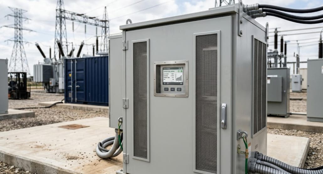
C-Rate and Discharge Duration
C-rate compares PCS power to battery energy. A 0.5C system runs at full power for 2 hours.
A 1C system, by contrast, runs for 1 hour instead. It also costs 20-40% more, since it needs bigger power electronics.
Past about 1.5C, systems often need liquid cooling too. Most 2-8 hour backup projects land in the 0.1C-0.5C range, which keeps cost down and favors longer cycle life.
Grid-Forming vs. Grid-Following PCS
A grid-following PCS needs a live voltage signal to sync to. It works for peak shaving, but not for a dead, powered-down site.
So true backup duty needs a grid-forming PCS, or a hybrid inverter with black-start. It must set voltage and frequency itself, the instant power drops.
Diesel Generator Replacement Sizing Calculator
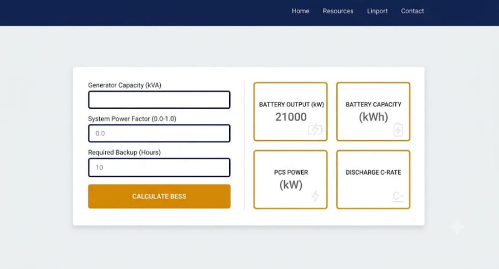
Use the free calculator below to size your site. Enter your generator’s kVA, power factor, and backup hours.
It converts kVA to real kW, then applies the formulas from this guide.
Diesel generator replacement calculator
Enter your generator’s rating and backup needs to get a starting BESS and PCS/inverter size. This is a budgetary estimate — confirm with a load study before procurement.
Advanced settings (DoD, efficiency, margins)
How the Calculator Works
To operate the calculator, simply enter your generator kVA, power factor, optional kW override, and required backup duration.
Additionally, advanced settings allow you to fine-tune depth of discharge, system efficiency, and safety margins.
First, your real load in kW. Second, a suggested BESS size in kWh. Third, a PCS size in kW, rounded to a standard size. Finally, the resulting C-rate.
| Input | Default | Purpose |
|---|---|---|
| Generator kVA | None, required unless using peak load override | Nameplate rating from the generator’s data plate |
| Power factor | 0.8 | Converts kVA to real kW |
| Peak load override (kW) | Blank | Use if you already have a measured kW figure |
| Backup hours needed | None, required | Sets the energy duration target |
| Depth of discharge | 90% | Usable portion of the battery’s rated capacity |
| Round-trip efficiency | 93% | Accounts for conversion losses |
| Energy safety margin | 20% | Buffer for load growth and inrush |
| PCS inrush margin | 25% | Buffer for motor and HVAC startup surge |
Case Studies: Diesel Generator Replacement with BESS in Practice
The examples below come from real 2026 deployments.
For more C&I projects, see Sunlith’s C&I BESS case studies roundup.
Case 1 — Diesel Generator Replacement at an Industrial Plant
An Indian market study covered a plant that kept its diesel generator. Instead, it added a behind-the-meter BESS rather than removing the genset.
So the battery handled daily outages with frequent cycling. The generator, meanwhile, stayed on standby for deeper outages.
A 1-hour BESS, sized to the average outage, paid back faster than a bigger system built for worst-case events. That is a lesson against over-sizing.

Case 2 — Solar + BESS Replacing Diesel at High Altitude (Leh, India)
Leh is a remote, high-altitude region of India. But it has long relied on diesel for backup power.
There, solar-plus-storage was rolled out to replace diesel at scale. The same study found this works even off-grid, once local power prices rise even a little.
This matches the pattern in Sunlith’s Island Grid BESS engineering guide. There, solar takes over as the main power source, and the BESS covers stability and overnight load.
Case 3 — Diesel Generator Replacement for a Telecom Tower Network
A telecom operator ran diesel gensets across remote towers. As a result, this meant high fuel bills and constant upkeep.
So the company switched to solar-plus-battery as the main power source at each site. Generators stayed on as backup only.
Fuel use dropped a lot. As a result, generator runtime fell, service intervals stretched out, and uptime improved.
Case 4 — Hospital Hybrid Backup (Australia)
A hospital in Australia added a BESS next to its diesel generators. Instead, it did not remove them.
This fits any site where power loss is a safety risk. The hybrid setup cut daily fuel use and backed up short outages without starting the genset.
How to Transition from Generator to BESS: A Phased Approach
- Audit the load: capture 12 months of interval data, or a representative outage load profile. Also, confirm whether backup covers full production or critical circuits only.
- Size the BESS and PCS independently: use the kWh formula for energy. Then size the PCS to peak kW, with an inrush margin.
- Install alongside the existing generator: commission the BESS in parallel, and do not decommission the genset until performance is proven.
- Run site acceptance testing: verify switching time, SLA compliance, and grid-forming black-start behavior under real load.
- Reclassify or retire the generator: once the BESS reliably carries day-to-day backup, shift it to a rarely-used secondary role. Or remove it from service entirely.
Key Takeaways on Diesel Generator Replacement
| Point | Why It Matters |
|---|---|
| Convert kVA to kW before sizing anything | Generators are rated in kVA; BESS kWh and PCS kW both depend on the real kW figure |
| Size energy (kWh) and power (kW) separately | An undersized PCS behind a large battery still fails to carry the load |
| Use Load x Hours x 1.43 as a starting formula | Bakes in a 1.2x safety margin, 90% DoD, and about 93% round-trip efficiency for LFP |
| Diesel costs $0.22-0.65/kWh all-in | Fuel alone runs $0.22-0.28/kWh at optimal load; maintenance pushes it higher |
| Grid-forming PCS is required for true backup duty | Grid-following inverters cannot black-start a de-energized site |
| Install BESS alongside the generator first | Every documented case study kept the genset as backup during commissioning |
| Typical payback is 4-7 years | Driven by avoided fuel spend, plus demand charge and peak-shaving revenue |
Frequently Asked Questions
Can a BESS completely replace a diesel generator?
Yes, for many sites. If outages run from minutes to a few hours, a well-sized BESS can fully replace the generator. It just needs a grid-forming PCS.
This also works if solar recharges the battery each day. But sites with life-safety loads, or rare, multi-day outages, often keep a generator as backup.
What is a realistic payback period for diesel generator replacement with BESS?
Most C&I projects pay back in 4 to 7 years. So this comes mainly from avoided fuel and upkeep cost.
It also comes from peak-shaving and demand-charge savings, on normal days with no outage.
Why does PCS sizing matter separately from battery kWh?
Battery kWh sets how long the system runs. PCS kW, by contrast, sets how much power it can push at once.
So an undersized PCS caps output, no matter how much energy sits in the battery.
How do I convert my generator’s kVA rating for BESS sizing?
Multiply the kVA rating by the power factor to get real kW. Most industrial sites run near 0.8 PF.
But check your generator’s data sheet to confirm. For example, 125 kVA at 0.8 PF equals 100 kW.
What battery chemistry works best for diesel generator replacement?
LFP is the standard choice for C&I diesel generator replacement. Also, it offers strong thermal stability and long cycle life.
It also carries no thermal runaway risk, unlike some other lithium types. This is the same reasoning behind Sunlith’s chemistry choice across its C&I line.