
UK BESS Grid Connection: G98, G99, NESO and Grid Code Guide
A UK BESS grid connection depends on the connection voltage, export capacity, site location, network operator, and the project’s status in the connections queue. Smaller distribution-connected systems commonly follow a DNO-led Engineering Recommendation G98 or G99 process. Larger embedded and transmission-connected projects, by contrast, may need more extensive system studies, Grid Code compliance, CUSC arrangements, and a place in the reformed connections process. So a battery is never approved just because its inverter rating matches the site.
Scope note: This guide covers BESS projects connecting in Great Britain (England, Scotland, and Wales), regulated by Ofgem and coordinated by NESO. Northern Ireland operates under a separate regulatory system, as part of the Single Electricity Market with Ireland, which this guide does not cover in detail.
Quick answer: A UK BESS grid connection depends on connection voltage, export capacity, location, and where the project sits in the connections queue. Smaller, distribution-connected batteries typically go through an Engineering Recommendation G98 or G99 application with the local DNO. Larger or transmission-connected projects usually need a Bilateral Connection Agreement, Grid Code compliance, and a place in NESO’s reformed connections pipeline.
So, this guide walks through:
- How NESO, Ofgem, DNOs and Transmission Owners each fit into a BESS interconnection
- The difference between distribution-connected (G98/G99/G100) and transmission-connected pathways
- The stage-by-stage connection process, including NESO’s 2025 Connections Reform
- Grid Code requirements for Electricity Storage Modules
- UK-specific technical challenges and common project risks
UK BESS Connection Checklist
- Identify the likely point of connection and confirm distribution versus transmission voltage.
- Check whether the proposed installation falls within the applicable G98 current limit and notification conditions.
- Confirm the project’s status and expected offer window under NESO’s Connections Reform pipeline.
- Screen local network constraint and curtailment risk for the specific region.
- Confirm the applicable Grid Code Power Generating Module Type and its technical requirements.
- Ask the PCS supplier and system integrator for the model format the network operator requires, such as RMS or EMT, together with validated parameters, controller logic, and operating-mode assumptions, before finalising procurement.
- Allow schedule contingency for studies, Bilateral Connection Agreement negotiation, and commissioning.
Who Governs a UK BESS Grid Connection?
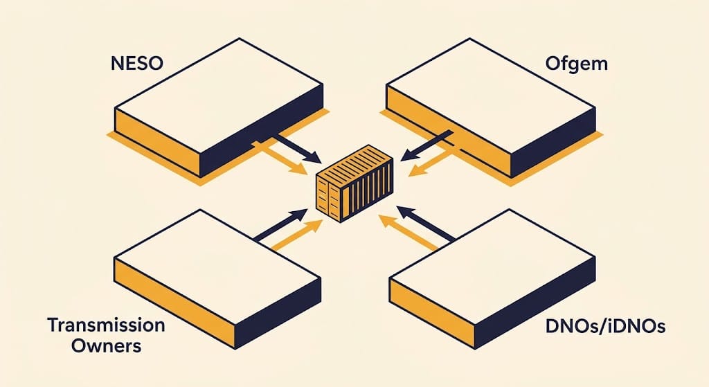
No single body runs UK BESS approval from start to finish. Instead, several organisations share the job, and the reformed connections process has changed how a few of them work together.
| Organisation | Main role for BESS projects |
| NESO | Great Britain’s electricity system operator. Coordinates the reformed transmission-connection process and works with Transmission Owners and DNOs on queue reform and connection offers. For many distribution-connected projects, the relevant DNO remains the main counterparty, not NESO directly. |
| Ofgem | Independent regulator for Great Britain. Approves code changes such as the Connections Reform modifications and regulates network company price controls. |
| Transmission Owners | Build and maintain the transmission network. Examples include National Grid Electricity Transmission (England and Wales), SP Transmission and Scottish Hydro Electric Transmission (Scotland). |
| DNOs and iDNOs | Assess and connect distribution-level projects. They process G98 and G99 applications, set local protection and export-limit conditions, and increasingly act as Distribution System Operators managing local network capacity. |
So don’t assume NESO reviews every battery project directly, and don’t assume it runs a single unified pipeline on its own. Smaller, distribution-connected batteries mostly deal with their DNO, so keep that relationship central throughout.
Current detail on each body’s role: NESO, Ofgem.
Distribution vs. Transmission: Two Paths for a UK BESS Grid Connection
One factor shapes grid approval more than any other: where the asset physically connects, and at what voltage. Distribution and transmission pathways lead to very different applications and timelines.
| Factor | Distribution-connected BESS | Transmission-connected BESS |
| Typical use case | C&I storage, community batteries, smaller grid-scale projects | Utility-scale storage, large co-located projects |
| Main counterparty | DNO or iDNO | NESO and the relevant Transmission Owner |
| Governing framework | EREC G98, G99, and G100 | Grid Code, CUSC, and a Bilateral Connection Agreement |
| Technical focus | Export limits, protection, voltage rise, anti-islanding | Power Generating Module Type, dynamic performance, system studies |
| Key risk | Local network constraint, DNO queue position | Connections Reform pipeline position, study timelines |
Project size alone doesn’t decide the pathway, though. A regional quirk matters here. In parts of Scotland, an embedded project as small as 30 MW can need a Bilateral Connection Agreement and CUSC party status. A similarly sized project in England or Wales, by contrast, may fall under the Licence Exempt Embedded Medium Power Stations arrangement instead. So confirm the specific threshold with the relevant network operator, rather than assuming a single GB-wide MW cut-off. More broadly, the categories in the table above are general planning distinctions, not universal legal classifications. A distribution-connected project can still carry Grid Code, CUSC, or transmission-system obligations depending on its configuration. So confirm the applicable route with the DNO, NESO, and the relevant Transmission Owner.
The UK BESS Grid Connection Process, Stage by Stage
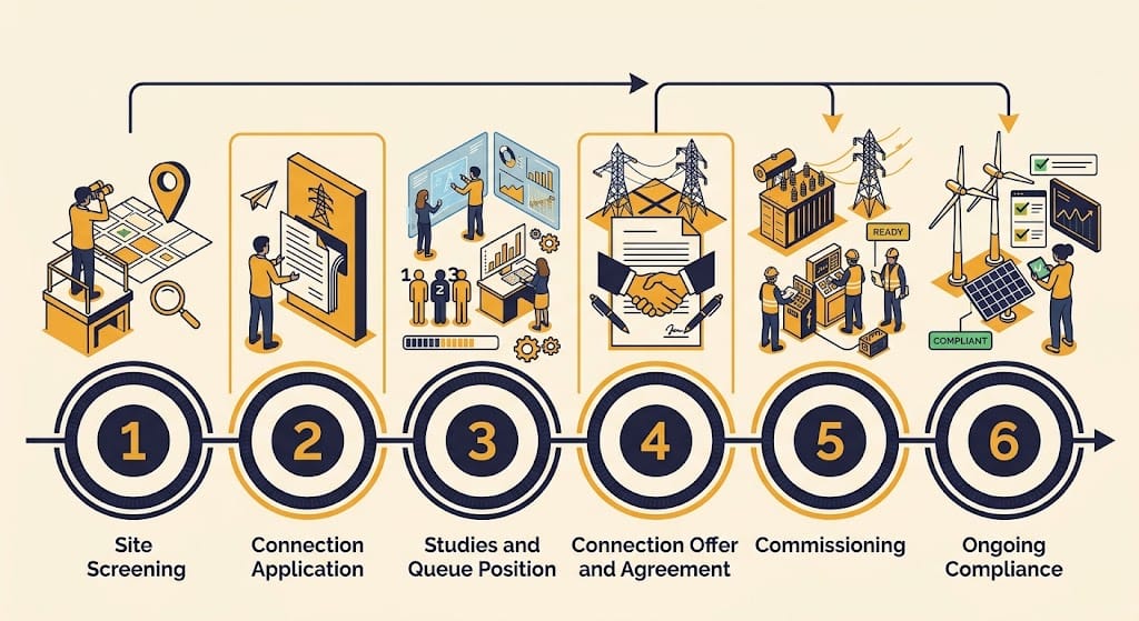
Treat the connection journey as a set of stages, not one checklist. Each stage builds on the last, and the 2025 Connections Reform changed how several of them work.
Stage 1: Site Screening and Capacity Assessment
First, check the site’s real limits before you lock in battery duration or PCS (power conversion system) rating. Review available capacity at the likely connection point. Then confirm whether the project falls within the applicable G98 current limit and notification conditions, or whether it will need a full G99 application instead. Next, assess local network constraint, since some regions are heavily congested for new BESS capacity, and a few areas have effectively closed for certain technologies.
Also map planning consent requirements and any land or grid-easement issues early. A connections queue position can take months to secure, so running planning and land work in parallel avoids a stacked delay later in the schedule.
Stage 2: Connection Application
Next, submit the applicable connection application. For distribution-connected projects, this usually means an EREC G99 application to the local DNO, identifying the proposed site, export capacity, inverter specifications, and intended operating modes. For larger or transmission-connected projects, this instead means an application to NESO. That application now sits inside the reformed Connections Reform pipeline, rather than the old first-come, first-served queue.
Stage 3: Studies and Queue Position
The network operator then sets the study scope for the project. Distribution-connected projects may need protection-coordination, voltage-rise, and export-limit studies. Larger or transmission-connected projects may also require load-flow, short-circuit, and dynamic-performance studies against the applicable Grid Code requirements.
Since 10 June 2025, eligible transmission-connected and some larger embedded projects are also assessed under NESO’s reformed connections framework, commonly known as TMO4+ (Target Model Option 4 Plus). Under this framework, a project earns a Gate 2 connection date and queue position by meeting defined readiness criteria and passing a strategic-alignment check. That replaces the old rule of holding a position by application date alone. Projects with existing agreements go through a one-off reassessment called Gate 2 to Whole Queue (G2TWQ). For small and medium embedded generators, NESO issues a Gate 1 offer to the DNO first, and the DNO takes it from there. The precise process depends on the project’s connection route, capacity, application status, and the relevant network operator. So confirm current requirements directly with NESO or the DNO, rather than assuming every project follows an identical path.
Stage 4: Connection Offer and Agreement
For distribution-connected projects, this stage produces the DNO’s response to a G98 or G99 application. Depending on the project and DNO process, that response may take the form of an acceptance, technical offer, connection offer, or approval subject to specific documentation. Either way, it sets out technical conditions and any required network reinforcement. For transmission-connected or larger embedded projects, this stage instead produces a Bilateral Connection Agreement. That agreement binds the project to the Connection and Use of System Code (CUSC) and the applicable Grid Code requirements. Offer timing now depends on the project’s phase and queue position under Connections Reform. So confirm current expectations directly with NESO or the relevant DNO, rather than relying on older published timelines.
Stage 5: Design, Construction and Commissioning
Commissioning confirms the installed plant matches the approved design. So, first, expect to provide as-built drawings and protection settings. Then witness testing and G99 or Grid Code compliance testing follow, covering protection, anti-islanding, and, where applicable, dynamic-performance verification. Commissioning evidence and updated models may also be required before the DNO or NESO issues final approval to energise.
Stage 6: Ongoing Compliance
Compliance does not stop once operation begins. Instead, changes to inverter firmware, protection settings, control-system configuration, or export limits may trigger a reassessment. So, treat compliance documentation as an ongoing operational task, not a one-off commissioning step, since it protects the connection agreement over the plant’s full operating life.
Realistic timelines vary widely by project size and location. A straightforward G98 or small G99 connection may progress in a matter of months. But a transmission-connected or large embedded project now depends heavily on its position in the reformed connections pipeline. NESO’s own December 2025 results show the queue moving in phases through 2026 and beyond. Build schedule contingency around queue position and study timelines, since both remain genuinely difficult to forecast precisely during this transition period.
Grid Code Requirements for a UK BESS Grid Connection
Grid Code requirements sit at the technical centre of any transmission-connected or large distribution-connected UK BESS grid connection. The Grid Code and associated connection-code provisions include requirements specifically relevant to Electricity Storage Modules. These interact with the applicable Power Generating Module classification, connection voltage, capacity, and operating mode.
First, the Grid Code sorts Power Generating Modules, including storage, into Types A to D. The thresholds are the same across Great Britain, and they set the technical requirements each module must meet. Then, depending on the module type and connection arrangement, a project may need to become a CUSC party. Or it may instead qualify for a licence-exempt arrangement handled mainly through the Distribution Code. Which pathway applies depends on connection voltage, project size, and sometimes regional variation. So confirm the applicable module type and compliance route directly with NESO or the relevant network operator early in development.
| Performance area | Why it matters for battery storage |
| Active-power control | The BESS must charge, discharge, and respond to dispatch instructions accurately. |
| Reactive-power capability | The plant may need to inject or absorb reactive power to support voltage. |
| Frequency response | Storage can respond fast, but the response must still match the relevant Grid Code obligations. |
| Fault ride-through | The plant may need to stay connected through defined voltage disturbances. |
| Protection | Settings must clear internal faults while avoiding unnecessary tripping for external events. |
| Dynamic performance | Validated models help confirm the plant behaves as designed under real system conditions. |
Background reading: NESO’s Guidance Notes for Electricity Storage EU Code Users.
Does Every BESS Need a Bilateral Connection Agreement?
No, not every project does. Whether a BESS needs a Bilateral Connection Agreement and CUSC party status instead depends on its connection voltage, capacity, and sometimes its specific region. The England/Wales-versus-Scotland threshold difference shows why. Smaller distribution-connected projects instead work through the relevant DNO under G98 or G99. Developers should confirm the applicable pathway during early site screening rather than rely on a single capacity threshold as a proxy.
G98, G99, and G100 for Distribution-Connected Batteries
For distribution-connected battery systems, Engineering Recommendations G98 and G99 are the core technical references, with G100 applying separately wherever export limitation is used. G98 covers connect-and-notify installations that meet specific current and equipment conditions, generally up to 16A per phase, roughly 3.68kW on a single-phase supply. Installations outside those conditions generally need a full G99 application, but the DNO should confirm the correct route for the proposed configuration rather than relying on capacity alone.
G100 applies where an export limitation scheme is used to restrict the power a site sends back to the distribution network. It is not specific to DC-coupled battery storage. A DC-coupled BESS may need to meet G98 or G99 requirements too, depending on the generating-unit and inverter configuration. And an export-limited connection normally needs a validated control scheme, metering arrangement, and fail-safe behaviour. The DNO needs to be able to rely on that behaviour if control, communications, or measurement fails. None of these Engineering Recommendations replace the DNO’s own connection agreement or local network conditions. Larger C&I or grid-scale battery projects should confirm export limits, protection requirements, and network reinforcement needs directly with the DNO. See our full BESS grid codes comparison for the country-by-country comparison, including how UK grid codes fit alongside other major markets.
Reference: ENA’s official G98/G99 forms and guidance.
Which UK BESS Connection Pathway Applies?
A quick self-check before diving into the detail below.
| Question | Likely implication |
| Is the system within the G98 current limit and notification conditions? | G98 connect-and-notify may apply |
| Is the system above those G98 limits or conditions? | A G99 assessment is likely |
| Does the project use an export limitation scheme? | G100-related requirements may apply, alongside G98 or G99 |
| Is the project transmission-connected or a large embedded project? | NESO, the Transmission Owner, CUSC, Grid Code, and BCA requirements may arise |
| Is the project in the reformed connections queue? | Gate 1 or Gate 2 status and readiness evidence may affect timing |
Technical Challenges Unique to a UK BESS Grid Connection
A few UK-specific conditions make grid approval harder here than a generic global playbook suggests. These conditions shape both design choices and realistic project timelines.
Connections Reform and Queue Position
As Stage 3 covers, readiness now matters as much as application date. NESO’s own reporting shows the pre-reform queue exceeded 700 GW, while the reformed pipeline instead prioritises a smaller, more deliverable set of projects. In practice, that means a project’s land rights, planning progress, and evidence pack can matter more to its timing than how early it applied.
See: NESO’s Connections Reform results.
Grid-forming capability: NESO has published dedicated technical guidance for grid-forming plant, including Electricity Storage Modules. In some locations, connection studies may consider whether grid-forming controls can support network stability. Grid-forming capability is not a substitute for a connection assessment, however. Its value depends on the network need, the plant’s control design, and the operating characteristics the project accepts. So treat it as one design input among several, not a fix on its own.
See: NESO’s Grid Forming Guidance Note.
Regional Network Constraint
Network capacity for new BESS varies sharply by region. Some parts of Great Britain, including areas of Scotland, face significant constraint for new storage and generation capacity. So, in practice, a site’s regional location can matter as much as its technical design for realistic connection timing.
Curtailment and Commercial Risk
A connection offer may include a formal non-firm connection, active network management, or another constraint mechanism in congested areas. These are not all the same thing. Distribution export limitations, transmission constraint costs, and scheduled or dynamic curtailment can each apply differently depending on the connection. Because of this, test your revenue model against the specific curtailment terms in your own connection offer, not a generic assumption. Do this before you finalise the business case. A conservative revenue case, built around the connection offer’s real terms, protects the project from an optimistic forecast that never eventuates.
Common Risks in a UK BESS Grid Connection
Most delays in a UK BESS grid connection trace back to a small set of repeat mistakes. So here is how to catch them early.
| Risk | Consequence | Mitigation |
| Assuming a single GB-wide MW threshold applies | Wrong compliance pathway assumed early | Confirm the applicable threshold with the specific network operator |
| Treating queue position as fixed by application date | Schedule built on outdated queue assumptions | Track readiness and Gate 2 status directly through NESO |
| Selecting a site before checking regional constraint | Unexpected non-firm terms or long delays | Screen regional network capacity early in site selection |
| Incomplete or unvalidated dynamic models | Delayed studies and commissioning rework | Require validated models from the PCS vendor and integrator |
| Treating Grid Code compliance as an afterthought | Design changes late in development | Confirm the applicable Power Generating Module Type early |
| Uncontrolled post-commissioning changes | Non-compliance or reassessment obligations | Set up formal change-control for firmware and protection settings |
Planning a BESS project in the UK? Start with a connection-readiness assessment. Cover site capacity, regional constraint, the applicable Grid Code or G98/G99 pathway, and Connections Reform queue status, before you finalise equipment specifications.
Frequently Asked Questions About a UK BESS Grid Connection
Common questions developers ask before signing a connection agreement, answered directly.
Do I need G98 or G99 for a battery storage system?
It depends on the maximum design current per phase and the connection arrangement, not just battery nameplate capacity. Systems that meet the G98 current limit and notification conditions, generally up to 16A per phase (roughly 3.68kW single-phase), can usually connect-and-notify. Systems outside those conditions generally need a full G99 application instead. The assessment timescale varies by DNO and project complexity, so treat any indicative period as a planning estimate, not a guaranteed service window.
What is NESO’s Connections Reform and how does it affect BESS projects?
Connections Reform, approved by Ofgem on 15 April 2025 and live from 10 June 2025, replaced the old first-come, first-served queue with the readiness-based TMO4+ model. Eligible projects earn a Gate 2 connection date by meeting readiness criteria and passing a strategic-alignment check, rather than by application date alone. Projects with existing agreements go through a one-off reassessment called Gate 2 to Whole Queue. The precise process still varies by connection route and network operator.
Does every large BESS project need a Bilateral Connection Agreement?
Not automatically. As the regional-threshold note above explains, it depends on connection voltage, capacity, and sometimes region. Confirm the applicable pathway with the relevant network operator during early screening, rather than assuming a fixed MW cut-off.
What is G100 and when does it apply?
G100 applies where an export limitation scheme is used to restrict how much power a site sends back to the distribution network. It is not specific to DC-coupled battery storage; a DC-coupled BESS may still need G98 or G99 separately, depending on its configuration. Confirm the applicable route with the DNO.
Does Northern Ireland follow the same rules as Great Britain?
No. Northern Ireland operates under a separate regulatory system, as part of the Single Electricity Market with Ireland, with its own versions of the equivalent engineering recommendations. This guide focuses on Great Britain.
How long does a UK BESS grid connection take?
It varies widely. A straightforward G98 or small G99 connection can take months. A transmission-connected or large embedded project now depends heavily on its position in the reformed connections pipeline, which is still moving through its phased rollout.
What is system constraint and how does it affect BESS projects?
Network constraint describes limited capacity at a given location to accept new generation or storage. In constrained areas, a connection offer may come with curtailment terms or a non-firm connection, which developers should factor into their revenue modelling.
Can a battery connect without full export capability in the UK?
Yes, in some cases. A non-export or export-limited design under G100 can simplify the connection pathway, especially for smaller distribution-connected projects. However, the project generally still needs DNO approval. It also needs a validated control scheme, metering arrangement, and fail-safe behaviour the DNO can rely on if control, communications, or measurement fails.
Glossary of Terms for This UK BESS Grid Connection Guide
Because this guide leans technical, here are the acronyms used throughout, defined in plain terms.
Organisations, Codes, and Agreements
BESS — Battery Energy Storage System — the battery, inverter, and control equipment that stores and dispatches electricity.
NESO — National Energy System Operator — Great Britain’s independent electricity system operator, responsible for coordinating the reformed transmission connections process.
Ofgem — The independent regulator for Great Britain’s gas and electricity markets, which approves code changes such as the Connections Reform modifications.
DNO — Distribution Network Operator — the regional company that owns and operates the local electricity distribution network.
iDNO — Independent Distribution Network Operator — a licensed operator of a distribution network not owned by the regional DNO, often serving a specific site or development.
TO — Transmission Owner — the company that builds and maintains the transmission network in its region, such as National Grid Electricity Transmission or SP Transmission.
CUSC — Connection and Use of System Code — the industry code governing transmission connection and use-of-system arrangements in Great Britain.
BCA — Bilateral Connection Agreement — the formal agreement binding a transmission-connected or large embedded project to CUSC and Grid Code requirements.
PGM — Power Generating Module — the Grid Code classification (Types A to D) based on connection voltage and capacity, which sets a project’s technical requirements.
ESM — Electricity Storage Module — the Grid Code and connection-code term for a battery storage installation, which interacts with the applicable PGM classification.
Connection Types and Process Terms
G98 — The Engineering Recommendation for connect-and-notify generation and storage installations that meet specific current and equipment conditions.
G99 — The Engineering Recommendation requiring DNO approval before connection, for installations that fall outside G98 conditions.
G100 — The Engineering Recommendation covering export and import limitation schemes, applicable wherever a project limits what it sends to or draws from the network.
TMO4+ — Target Model Option 4 Plus — the readiness-based connections queue model introduced under the 2025 Connections Reform.
Gate 1 — An indicative connection offer stage, typically issued to the DNO for small and medium embedded generators under the reformed process.
Gate 2 — The stage at which a project earns a confirmed connection date, point of connection, and queue position, after meeting readiness and strategic-alignment criteria.
Important: This guide is general information, so treat it that way, not as legal, engineering, or connection advice. Grid-compliance requirements vary by network operator, project design, location, and the applicable rules at the time of assessment. The UK’s connections framework is also under active reform. Confirm requirements with the relevant DNO, NESO, Ofgem where applicable, and qualified electrical, grid-connection, and legal advisers.
Further Reading on UK BESS Grid Connection
More Sunlith Energy guides on battery storage connection, interconnection, and compliance.
- BESS interconnection process (BESS Interconnection Process: From Application to Commercial Operation)
- UK and international BESS grid-code requirements (BESS Grid Codes and Compliance)
- Australia BESS grid connection process (Australia BESS Grid Connection: AEMO, TNSP and DNSP Requirements)
- PCS fault ride-through and LVRT/HVRT capability (Fault Ride-Through Features: The PCS Hardware and Control Functions Behind LVRT/HVRT Compliance)
- Voltage ride-through curves behind Grid Code compliance (LVRT and HVRT: Voltage Ride-Through for BESS and Solar)
Source
Grid Code and Connections Reform detail in this guide is grounded in NESO’s Connections Reform overview.
Australia BESS Grid Connection: AEMO, TNSP and DNSP Requirements
Every Australia BESS grid connection follows its own path. There is no single national checklist. Requirements vary by jurisdiction, network provider, connection voltage, and project size. They also depend on system strength and whether the asset trades in the National Electricity Market. So a battery is never approved just because its inverter rating matches the site. Developers must also show the whole plant stays stable under normal and disturbed grid conditions.
Scope note: This guide focuses primarily on BESS projects connecting in the National Electricity Market (NEM), covering Queensland, New South Wales, the ACT, Victoria, South Australia and Tasmania. Western Australia and the Northern Territory operate separate electricity-market and network-connection arrangements, which this guide does not cover in detail.
Quick answer: An Australia BESS grid connection depends on several things: connection voltage, export and import capacity, location, market participation, and the rules of the relevant network. Large, NEM-connected projects usually undergo detailed connection studies and project-specific performance-standard assessment. Smaller systems typically work with their DNSP, but may still need export controls, protection upgrades, or network-specific approval.
This guide walks through:
- How AEMO, AEMC, AER, TNSPs and DNSPs each fit into a BESS interconnection
- The difference between transmission- and distribution-connected pathways
- The stage-by-stage connection process, including Generator Performance Standards
- Australia-specific technical challenges, including system strength and control interactions
- Common project risks and how to reduce them
Australia BESS Connection Checklist
- Identify the likely point of connection and available import/export capacity.
- Confirm whether the project is transmission-connected, distribution-connected, embedded, or behind the meter.
- Screen local fault level, system strength, congestion, and curtailment risk.
- Confirm the relevant registration, performance-standard, and connection-agreement pathway.
- Obtain required OEM and integrator RMS and EMT model commitments before procurement.
- Define the interface between the PCS, PPC, EMS, protection scheme, SCADA, and DNSP/TNSP controls.
- Allow schedule contingency for study iterations, technical negotiations, remediation works, and commissioning evidence.
Who Governs an Australia BESS Grid Connection?
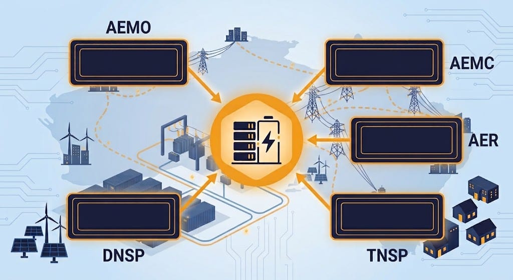
No single regulator runs the approval process start to finish. Instead, several bodies share the job. Each one controls a different part of the connection.
| Organisation | Main role for BESS projects |
| AEMO | Operates the NEM and administers registration and connection-related processes under the National Electricity Rules. Its role in a given project depends on the asset’s registration status, connection pathway, and applicable performance-standard requirements. |
| AEMC | Writes the National Electricity Rules. These govern connection and market arrangements. |
| AER | Regulates network businesses and market conduct. |
| TNSPs | Assess connection applications, define required studies and technical conditions, and execute the connection agreement for transmission-scale projects. Examples include Transgrid, Powerlink, ElectraNet, AusNet and TasNetworks. |
| DNSPs | Assess connection applications, define required studies and technical conditions, and execute the connection agreement for distribution-connected projects. They also set local protection, metering and export-limit rules. |
| WA and NT bodies | Operate under separate market and regulatory structures, outside the NEM. |
Don’t assume AEMO approves every battery. Instead, its role depends on the connection pathway and the project’s registration status. Either way, the connecting network business stays central to approval, so keep that relationship close throughout.
Current detail on each body’s role: AEMO, AEMC, AER.
Transmission vs. Distribution: Two Paths for an Australia BESS Grid Connection
One factor shapes grid approval more than any other: where the asset physically connects. Transmission and distribution pathways lead to very different studies and timelines. So, picking the right connection point early saves real time later.
| Factor | Transmission-connected BESS | Distribution-connected BESS |
| Typical use case | Utility-scale storage, renewable-plus-storage, grid-support assets | C&I storage, community batteries, smaller utility projects |
| Main counterparty | TNSP | DNSP |
| Market relevance | Usually significant for registered NEM participants | May be exempt, embedded, or export-limited |
| Technical focus | Performance standards, system strength, network-wide models | Export capacity, protection, voltage rise, local feeders |
| Key risk | Long study cycles, changing negotiations | Limited export capacity, local upgrade costs |
A behind-the-meter battery is not automatically simple, though. For example, if it can export, island, or materially alter site demand or network flows, the DNSP may still get involved. It can ask for studies, protection changes, or new operating limits.
The Australia BESS Grid Connection Process, Stage by Stage
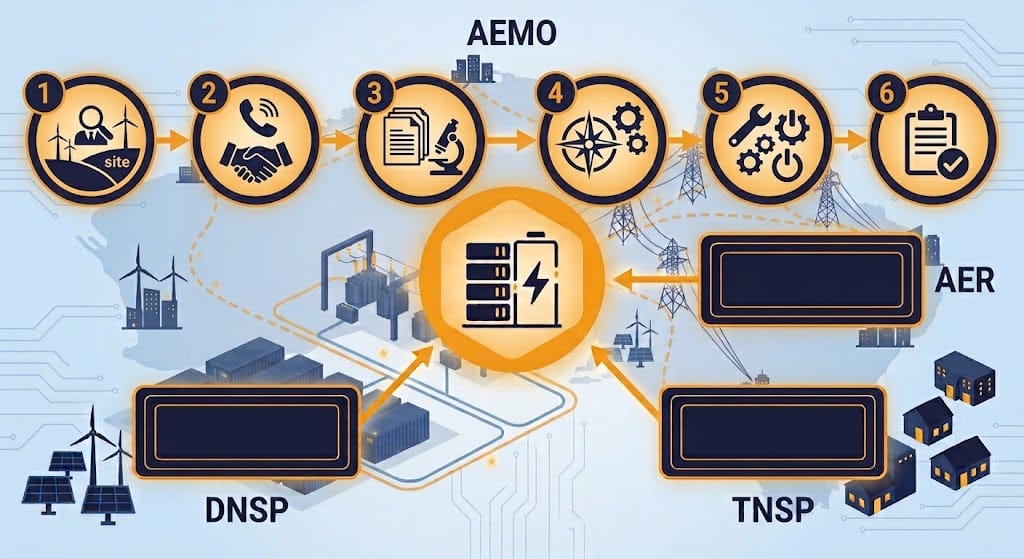
Treat the connection journey as a set of stages, not one checklist. Each stage builds on the last. Skipping ahead usually costs time later.
Stage 1: Site Screening and Capacity Assessment
First, check the site’s real limits before you lock in battery duration or PCS (power conversion system) rating. Review available import and export capacity. Then confirm the connection voltage and the likely point of connection. Next, assess local fault levels, system strength, and nearby renewable congestion. Also check curtailment risk early, since it directly affects revenue.
Finally, decide whether the project will run non-exporting, export-limited, or under a dynamic operating envelope. Dynamic operating envelopes are an emerging and increasingly used option on parts of Australian distribution networks. Instead of a fixed export limit, some networks now offer a time-varying limit based on real conditions. Availability, control interfaces, and commercial implications vary by DNSP and connection type, so confirm what your specific network actually offers.
Also map the site’s land tenure, easements, and any planning-approval overlap early. A grid study can take months, so running it in parallel with land and environmental approvals avoids a stacked delay later in the schedule.
More on how dynamic operating envelopes work: ARENA’s Dynamic Operating Envelopes work.
Stage 2: Initial Connection Enquiry
Next, submit a connection enquiry to the relevant network provider. The enquiry should identify the proposed site, point of connection, MW/MWh rating, intended operating modes, and requested import and export limits. Include the preliminary single-line diagram, inverter and transformer specifications, and any planned participation in energy, FCAS, demand-response, or backup-power functions.
Stage 3: Connection Studies
The network provider then sets the study scope for the project. Larger or more complex assets may require load-flow, short-circuit, harmonic, protection-coordination, and reactive-power studies. Where the connection is electrically weak, or where inverter interactions are material, the assessment may also require dynamic RMS (electromechanical, phasor-domain simulation) and EMT (electromagnetic-transient simulation) modelling.
Treat model submission as real engineering, not paperwork. The network assessment may depend on models for the PCS, plant power controller, EMS interfaces, transformers, protection systems, and the integrated BESS plant, not the PCS alone. Require the relevant OEMs and system integrator to supply validated RMS models and, where required, EMT models compatible with the relevant NSP or AEMO study environment, before finalising supply contracts.
For a deeper look at how these study types work in general, see our BESS grid connection studies guide.
Stage 4: Generator Performance Standards Negotiation
For projects subject to the applicable NER performance-standard framework, this stage establishes the plant’s Generator Performance Standards. These obligations are developed through the connection process with the connecting TNSP or DNSP, with AEMO involved where the National Electricity Rules require it. GPS is not a generic battery standard: it reflects the applicable rules, the site’s network conditions, and the final BESS design. Negotiation can run for several months on a complex site, so start the GPS conversation well before financial close, not after it.
Stage 5: Design, Construction and Commissioning
Commissioning confirms the installed plant matches the approved design. So, first, expect to provide as-built drawings and protection settings. Then factory or site acceptance test results come next, along with SCADA testing and metering verification. Commissioning may also include verification of fault-ride-through performance, where required under the agreed performance standards or connection agreement, alongside functional testing, telemetry checks, protection validation, model updates, and the evidence needed to demonstrate compliance.
Stage 6: Ongoing Compliance
Compliance does not stop once operation begins. Instead, battery augmentation, changes to inverter/PPC/EMS settings, control firmware, protection settings, or approved import/export limits may trigger reassessment. So, treat compliance documentation as an ongoing operational task, not a one-off commissioning step.
Realistic timelines vary widely by project size and network congestion. A straightforward small distribution connection may progress in a matter of months, but schedules vary materially with DNSP processes, export capacity, engineering studies, protection works, metering, and construction requirements. A large, transmission-connected asset with system-strength studies can take a year or longer, especially if GPS negotiation runs through several rounds. Build schedule contingency around the studies stage, since it is the hardest part to forecast.
Generator Performance Standards for an Australia BESS Grid Connection
Generator Performance Standards sit at the technical centre of any Australia BESS grid connection. AEMO’s framework uses minimum and automatic access standards, plus a negotiated tier in between.
First, a minimum access standard is the lowest bar a plant must clear to connect at all. Then an automatic access standard sets a higher bar. Once met, it generally avoids detailed negotiation on that item. Where the rules permit, a negotiated standard may sit between the two. That still depends on the connection assessment process, the National Electricity Rules, the connecting network service provider, and AEMO’s role where applicable.
| Performance area | Why it matters for battery storage |
| Active-power control | The BESS must charge, discharge, and follow dispatch instructions accurately. |
| Reactive-power capability | The inverter may need to inject or absorb reactive power to support voltage. |
| Voltage control | Poorly tuned controls can create oscillations or conflict with nearby plant. |
| Frequency response | BESS reacts fast, but the response must still match market and network rules. |
| Fault ride-through | The plant may need to stay connected through defined voltage disturbances. |
| Protection | Settings must clear internal faults, but avoid tripping for external disturbances. |
| System strength | Weak grids can destabilise inverter controls, so site-specific studies matter. |
Background reading: AEMO’s Access Standard Assessment Guide.
Does a BESS Need AEMO Registration or GPS?
Not every battery follows the same pathway. Registration and performance-standard requirements depend on factors such as capacity, connection point, export capability, participant category, exemptions, and planned NEM participation. Developers should determine the applicable pathway during early grid screening rather than rely on a single capacity threshold as a proxy. Confirm the applicable pathway early with the relevant network service provider, AEMO, and specialist advisers.
AS/NZS 4777 and Distribution-Connected Batteries
For eligible low-voltage inverter energy systems, AS/NZS 4777 is a core grid-connection reference. Part 1 addresses installation and connection requirements, while Part 2 covers inverter functions, including anti-islanding behaviour.
However, AS/NZS 4777 does not replace the relevant DNSP’s connection process. Commercial, export-capable, or medium-voltage BESS projects may require additional protection studies, power-quality assessment, communications, metering, control functions, and formal commissioning evidence. This guide focuses on the AEMO/TNSP/DNSP interconnection process, not the installation-standard detail. See our full compliance-stack breakdown for that layer instead. Even a small C&I battery benefits from an early DNSP conversation, since export limits and metering requirements vary widely between networks.
Reference: AEMO’s AS/NZS 4777.2 inverter requirements overview.
Technical Challenges Unique to an Australia BESS Grid Connection
A few local conditions make grid approval harder here than a generic global playbook suggests. These challenges shape both design choices and approval timelines.
System Strength and Weak-Grid Performance
Many Australian renewable and storage projects sit in weak-grid areas. Often, other inverter-based plant sits nearby too. So a BESS must do more than hit its MW and MWh targets. Its controls must also stay stable through voltage disturbances and changing grid impedance.
See: AEMO’s System Strength Impact Assessment Guidelines.
Grid-forming capability: In some locations, connection studies may consider whether grid-forming controls can improve system strength, voltage stability, restoration capability, or network resilience. Grid-forming capability is not a substitute for a connection assessment, however. Its value depends on the network need, the BESS control design, protection coordination, and the operating obligations the project accepts.
See: AEMO’s Grid-Forming BESS Connections fact sheet.
Control Interactions Between Assets
A single compliant inverter does not guarantee a compliant power plant. Instead, the combined behaviour of the PCS, plant power controller (PPC), and EMS (energy management system) matters just as much. Similarly, the behaviour of any nearby solar inverters or STATCOMs also plays a part. A hybrid site with both BESS and solar needs coordinated tuning across every controller, or one asset’s response can undermine an-other’s.
Curtailment and Dynamic Operating Envelopes
A connection offer may include export limits or constrained operation at certain times. Because of this, test your revenue model against reduced export, charging restrictions, and delayed network upgrades. Do this before you finalise the business case. A conservative revenue case, built around the connection offer’s real limits, protects the project from an optimistic forecast that never eventuates.
Common Risks in an Australia BESS Grid Connection
Most delays in an Australia BESS grid connection trace back to a small set of repeat mistakes. So here is how to catch them early.
| Risk | Consequence | Mitigation |
| Selecting a site before grid screening | Unexpected upgrade cost or limited export capacity | Screen capacity, fault level and system strength early |
| Designing around nominal inverter capability | Failure to meet site-specific dynamic performance | Validate PCS capability against grid studies first |
| Incomplete or unvalidated OEM models | Delayed studies and commissioning rework | Require validated RMS and EMT models in contracts |
| Treating GPS as an afterthought | Design changes late in development | Start GPS strategy during concept design |
| Underestimating DNSP requirements | Delays for C&I or embedded projects | Engage the DNSP before finalising system rating |
| Uncontrolled post-COD changes | Non-compliance or re-registration obligations | Set up formal change-control for firmware and settings |
Planning a BESS project in Australia? Start with a connection-readiness assessment covering site capacity, import and export limits, system strength, required studies, and compliance documentation, before you finalise equipment specifications.
Frequently Asked Questions About an Australia BESS Grid Connection
Common questions developers ask before signing off on a connection agreement, answered directly.
Does every BESS project need AEMO registration?
No, not automatically. It depends on project size, connection type, participant category, exemptions, and market participation. Larger NEM-facing assets are more likely to carry AEMO registration. Smaller, behind-the-meter systems mainly deal with their DNSP instead. Either way, confirm the applicable pathway early, since it shapes the whole approval process.
What is the most common mistake in a BESS interconnection project?
Locking in a site or equipment before confirming real import and export capacity and system strength. Screening should always come first. Procurement comes second.
Can a BESS connect in Australia without export capability?
Yes, it can. A non-export or export-limited design is possible, especially for C&I projects. However, the project generally still needs the relevant DNSP’s approval, connection agreement, or confirmation of its non-export arrangement, and controls that enforce the approved limit.
Why do EMT models matter for Australian BESS projects?
EMT models capture fast inverter behaviour that standard RMS models can miss. This matters most in weak-grid areas, where several inverter-based resources sit close together. In short, an EMT model gives the network confidence the plant will behave as designed under real disturbances.
Can a battery provide both backup power and grid services?
Potentially, yes, but only with careful design. In practice, the electrical architecture, islanding logic, and network agreement must all support both functions from the start.
What grid studies does a BESS need in Australia?
The required studies depend on the connection point and network conditions. A project may need load-flow, short-circuit, protection-coordination, harmonic, reactive-power, RMS, and EMT studies. Larger or weak-grid projects usually need a broader assessment than a low-voltage behind-the-meter battery.
What is system strength for a BESS project?
System strength describes how well the network can hold voltage steady and support stable inverter operation during a disturbance. In weak-grid areas, BESS controls may need extra validation through dynamic and EMT studies, and the project may face operating constraints or remediation requirements.
Can a BESS connect at medium voltage in Australia?
Yes. Many commercial and industrial or larger embedded BESS projects connect at medium voltage. These projects generally follow the relevant DNSP’s embedded-generation or connection process and may need more detailed studies and protection design than a low-voltage system.
Glossary of Terms for This Australia BESS Grid Connection Guide
A few acronyms used throughout this guide, defined in plain terms.
PCS — Power Conversion System — the inverter and control hardware that converts DC battery power to AC grid power.
EMS — Energy Management System — the software layer that dispatches and optimises battery operation.
PPC — Plant Power Controller — coordinates multiple inverters and assets at plant level.
RMS — Root Mean Square, or phasor-domain, simulation model used to assess slower power-system and plant-control dynamics.
EMT — Electromagnetic Transient simulation model used to assess fast inverter, protection, and control-system behaviour.
Important: This guide is general information, so treat it that way, not as legal, engineering, or connection advice. Grid-compliance requirements vary by network, project design, location, market participation, and the applicable rules at the time of assessment. Confirm requirements with the relevant DNSP or TNSP, AEMO where applicable, and qualified electrical, grid-connection, and legal advisers.
Further Reading on Australia BESS Grid Connection
More Sunlith Energy guides on battery storage connection, interconnection, and compliance.
- Learn the full BESS interconnection process (BESS Interconnection Process: From Application to Commercial Operation)
- Explore BESS grid-code requirements and compliance (BESS Grid Codes and Compliance)
- Review Australia’s 2026 BESS compliance stack (Australia’s New Battery Rules: The 2026 Compliance Stack)
- Understand PCS fault ride-through and LVRT/HVRT capability (Fault Ride-Through Features: The PCS Hardware and Control Functions Behind LVRT/HVRT Compliance)
- Review BESS short-circuit protection design (BESS Short-Circuit Protection)
Source
Generator Performance Standards detail in this guide is grounded in AEMO’s Access Standard Assessment Guide.
Indoor Battery Installation Regulations by Country and Code
Indoor battery installation regulations differ by country, and often by state, province, or city within that same country. Because of this, a lithium battery system approved for sale in one market isn’t automatically approved for indoor installation there.
Two separate questions decide compliance. First, does the hardware meet a recognized safety standard? Second, is it sited, separated, and protected correctly for that room, under the code edition the local area has actually adopted?
This guide is for ESS manufacturers, distributors, installers, developers, and facility owners, and covers residential, commercial, and light-industrial indoor installations. Even so, it is not a substitute for project-specific engineering, code review, or sign-off from the authority having jurisdiction (AHJ).
Quick Answer
Indoor lithium-ion battery storage must meet the electrical, building, and fire-safety rules where the project sits. It must also meet the certification terms tied to that product. System certification and fire-test data support compliance. Neither replaces project-specific design review or sign-off from the authority having jurisdiction (AHJ).
Important
This article gives a high-level regulatory overview. It is not engineering, legal, fire-safety, or permitting advice. Rules depend on the locally adopted code edition. They also depend on ESS chemistry and capacity, building occupancy, manufacturer instructions, product listing, and the local authority’s judgment. Confirm project rules with qualified local professionals before installation.
Why Indoor Battery Installation Regulations Vary by Country
Every framework below regulates the same failure mode: a lithium cell in thermal runaway releases heat, flammable off-gas, and, in a confined space, pressure.
What differs is how each system of codes assigns responsibility for that risk. Some lean on cell-level certification. While others lean on system-level test data, installation separation rules, building and fire code, or a mix of all four. For example, the U.S. National Fire Protection Association publishes the installation standard most American areas reference. Its scope shows how differently one country can frame the same physics problem.
Quick Reference: Indoor Battery Installation Regulations by Region
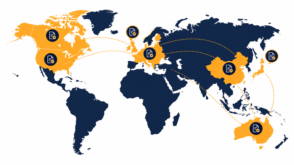
The table below summarizes each market’s main framework, plus the key product evidence and the practical sign-off authority.
| Region | Main installation framework | Key product/system evidence | Practical approval authority |
|---|---|---|---|
| United States | NFPA 855 (where adopted), IFC/IBC rules, NEC Article 706 | UL 9540 listing; UL 9540A test data where required | Local AHJ |
| Canada | Canadian Electrical Code (CSA C22.1), provincial/territorial codes | ANSI/CAN/UL 9540; ANSI/CAN/UL 1973 where applicable | Provincial or municipal authority |
| European Union | National electrical, building, and fire rules | IEC 62619 and related EN standards; CE conformity | National or local regulator |
| Germany | National rules plus VDE practice | IEC standards and VDE-AR-E 2510-50 where specified or expected | Installer, insurer, local authority |
| United Kingdom | PAS 63100, BS 7671 Chapter 57, relevant building/fire rules | Relevant product standards and installer paperwork | Installer, building control, MCS scheme rules |
| Australia / NZ | AS/NZS 5139 plus electrical/grid standards | Relevant battery and inverter certifications | Licensed installer and local regulator |
| China | GB 51048, GB/T 42288 — mainly station-scale | Certification path varies by product category; verify locally | Local fire and regulatory authorities |
| Japan | Fire Service Act, Electrical Appliances and Materials Safety Act | Product-specific METI/PSE/JIS/IEC review | Local fire authority and relevant regulator |
Treat the China and Japan rows as directional starting points, not final answers, because those sections below explain why.
United States: NFPA 855, UL 9540A, and NEC Article 706
UL 9540A Is a Test Method, Not a Certification
UL 9540A evaluates thermal-runaway fire propagation through escalating test levels: cell, module, unit, and, where needed, installation-level testing.
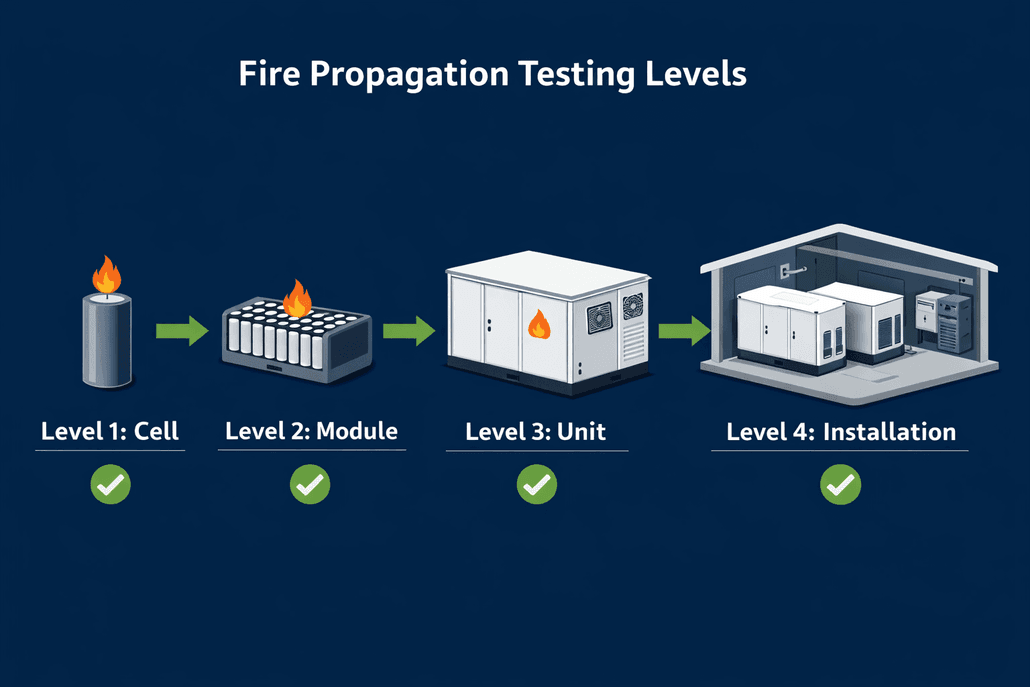
Its reports give product-specific fire and gas-release data. For example, engineers and the AHJ may use it to check spacing, aggregation, explosion control, ventilation, and fire-protection measures. That data informs the design and the AHJ’s decision. But it doesn’t replace the installation code or substitute for AHJ sign-off.
NFPA 855 Sets the Installation Rules
NFPA 855, Standard for the Installation of Stationary Energy Storage Systems, is the installation-level standard most U.S. areas reference for separation and fire-protection rules.
The 2026 edition, where adopted, significantly expands the default requirement for a documented Hazard Mitigation Analysis (HMA). “Where adopted” matters here, since code adoption is local and areas can lag the current edition by a cycle or more. So design to whichever edition the specific AHJ has actually put into force, not the newest one published.
NEC 706 Governs the Electrical Side
NEC Article 706, within NFPA 70, governs disconnects, labeling, and interconnection, no matter indoor or outdoor placement.
The International Fire Code and International Building Code incorporate NFPA 855 by reference in most adopting areas. But the AHJ still has final say. As a result, rulings vary between otherwise-similar properties depending on room construction and proximity to occupants.
Canada’s Indoor Battery Installation Regulations: Electrical Code and UL/CSA Marks
Canadian installation rules come from the Canadian Electrical Code (CSA C22.1), together with provincial or territorial electrical and fire codes, local authority rules, and the product’s certification and listing terms.
Recent editions of CSA C22.1 address energy storage systems in Section 64. Updates add a dedicated subsection for homes and raise the permitted capacity for a single residential ESS compared with earlier editions.
NFPA 855 may serve as a project, insurer, or engineering benchmark in some circumstances. But Canada’s code-adoption system is provincial and territorial, so don’t present NFPA 855 as a universally adopted Canadian installation standard. Instead, confirm the relevant provincial fire code for any specific project.
Product Certification: ANSI/CAN/UL 9540 and 1973
Product-level safety runs through the shared ANSI/CAN/UL 9540 (system) and ANSI/CAN/UL 1973 (battery) standards. A single test program can support evaluation for both the U.S. and Canadian markets.
Certification still has to come from an accredited body and be accepted by the relevant local authority. So don’t assume a U.S. listing alone is sufficient for a Canadian installation; confirm the Canadian mark or equivalent acceptance first.
European Union: IEC 62619 as the Base, Plus National Overlays
At the EU level, IEC 62619 anchors product safety for stationary lithium battery systems as the cell- and battery-level safety standard. Meanwhile, shared standards cover the power conversion and control gear, commonly cited alongside EN 62477 (power electronics) and EN 62109 (PV inverter safety, for hybrid systems).
CE marking demonstrates compliance with the relevant EU directives, but it is not itself an installation permit. Instead, siting, separation, and fire protection get set at the national or municipal level. This is where the EU differs most from the U.S. model of one widely referenced installation standard.
Germany’s Indoor Battery Installation Regulations: The VDE-AR-E 2510-50 Overlay
Germany is the clearest example of a national overlay with real market weight: VDE-AR-E 2510-50 sets safety rules for stationary lithium battery storage across its full lifecycle, from storage and transport through installation, operation, and end-of-life.
It’s commonly requested or expected in parts of the German residential and light commercial market. There, installers and some insurers treat it as a practical benchmark alongside the underlying IEC standards.
A product tested to VDE-AR-E 2510-50 may satisfy some expectations in other EU member states. But that doesn’t establish compliance with another country’s installation rules. Each national or local framework still needs its own check.
United Kingdom’s Indoor Battery Installation Regulations: PAS 63100, BS 7671, and MCS
The UK’s domestic battery framework combines fire-siting guidance, electrical-installation rules, product standards, and installer-scheme rules, built up in stages rather than as one document.
PAS 63100 and BS 7671 Chapter 57
PAS 63100:2024 provides domestic battery fire-safety guidance covering siting, fire separation, and detection, and is understood to treat bedrooms and unprotected escape routes as unsuitable locations.
A 2026 amendment to BS 7671 introduced Chapter 57, covering stationary secondary battery installations, and references PAS 63100 for domestic siting. Even so, installers should verify the exact current wording of that cross-reference against the licensed standard rather than relying on a summary.
MCS and the IET Code of Practice
MCS, the scheme relevant to specific UK incentive and export-payment programs, sets its own battery storage installation standard (MIS 3012). This points installers to the current edition of the IET Code of Practice for Electrical Energy Storage Systems.
The Code of Practice is the document that recommends following PAS 63100 for domestic siting. Because amendment and scheme language can change between code cycles, confirm the exact current rules against the licensed BS 7671 text and current MCS paperwork.
Australia and New Zealand: AS/NZS 5139
AS/NZS 5139 is Australia and New Zealand’s dedicated installation and safety standard for battery energy storage, covering siting, separation, ventilation, and protection rules in one document. By contrast, the UK and Canada use a multi-document approach.
It works alongside the broader inverter and grid-connection standards that already govern solar-plus-storage installs in the region. For the full detail on Australia’s compliance stack, including AS/NZS 4777.2 and AS/NZS 3008.1.1, see our dedicated Australian compliance hub.
China: Verify Scope and Certification Pathway Before Relying on a Summary
China’s framework for electrochemical energy-storage stations includes GB 51048 for design and GB/T 42288 for safety. Though both are principally relevant to station-scale projects rather than ordinary residential installations.
Rules for smaller indoor systems also depend on low-voltage electrical rules, product certification paths (CQC or CCC, depending on category), local fire-authority practice, and provincial rollout.
This is an area where a general summary is genuinely risky. So confirm the current edition, effective date, and scope threshold of GB 51048 with a qualified China-market compliance adviser. Also confirm whether your product category requires CCC, CQC, or another pathway before market entry. Always work from current Chinese-language official standards before any market-entry decision.
Japan: Fire Service Act Classification and Product-Specific Certification
Japan’s regulatory starting point differs from the markets above. Under the Fire Service Act, lithium-ion battery electrolyte can classify as a hazardous flammable liquid. The specific regulatory treatment depends on electrolyte composition, quantity, and the relevant hazardous-materials classification. So it isn’t a single blanket rule applied identically to every product.
METI, PSE, and IEC 62133-2
At the product level, certification runs through Japan’s METI framework. PSE marking under the Electrical Appliances and Materials Safety Act also applies. Both are product-specific rather than a blanket ESS-system certification comparable to UL 9540.
IEC 62133-2 may apply to certain portable or small stationary battery products. But don’t treat it as a general ESS system-level compliance pathway without confirming its applicability to the specific product and category under Japan’s rules.
Japan has no single dedicated residential-BESS installation standard like NFPA 855 or PAS 63100. Instead, it leans on the Fire Service Act’s hazardous-materials framework and local fire-authority discretion. This makes early talk with the local fire department a central part of Japanese project planning. Because of this, manufacturers should get Japan-specific regulatory review rather than treat PSE or IEC 62133-2 as a universal sign-off route.
What’s Consistent Across Every Country’s Indoor Battery Installation Regulations
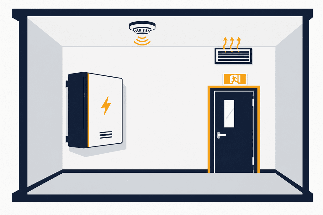
Underneath the different document names, every framework above answers the same five questions. So it’s worth designing to all five no matter which area’s paperwork sits on top.
Where Can the Unit Go?
Many frameworks impose tighter restrictions around bedrooms, escape routes, and high-occupancy areas. While garages, plant rooms, and detached structures usually face fewer limits. Because the exact restriction, and how it’s enforced, varies, check it against the locally adopted rules rather than assuming.
How Much Aggregate Capacity Is in the Room?
Several frameworks cap the sum of every unit present, not the rating of a single unit. That’s why systems added in stages sometimes fall out of compliance without anyone re-checking.
How Will an Early Fault Get Detected?
Depending on the system, occupancy, room layout, and local code, this may involve smoke detection, heat detection, battery-management-system alarms, off-gas detection, or a mix. Off-gas detection is increasingly considered for enclosed lithium-ion systems. But it isn’t a universal requirement across every area and product category.
What Fire Protection Fits This Specific Product?
This is where system-level test data, such as UL 9540A results or VDE-AR-E 2510-50 test reports, earns its keep: it can support a project-specific risk review and design choice. Instead, this avoids defaulting to the most conservative, most expensive option automatically.
Who Signs Off, and What Do They Need to See?
Whether it’s a U.S. AHJ, a UK MCS-certified installer working to PAS 63100, or a fire department talk under Japan’s Fire Service Act, every market ends the same way: the responsible authority or a qualified professional confirms project-specific compliance. No rulebook applies itself automatically.
A Practical Workflow for Meeting Indoor Battery Installation Regulations
Follow these six steps below for any indoor battery project, no matter the market.
- Identify the exact installation country, state or province, municipality, and building occupancy type. Rules can differ between neighboring areas in the same country.
- Confirm the locally adopted edition of the relevant electrical, building, and fire codes. Publication of a new standard edition doesn’t mean every area has adopted it yet.
- Confirm the product has the required system-level listing and component certifications for that specific market, not just the market where it was originally developed or tested.
- Review the manufacturer’s installation instructions, listing conditions, and any relevant UL 9540A (or equivalent) fire-test evidence referenced in the product’s certification.
- Assess aggregate installed energy, room configuration, egress proximity, ventilation, and fire-protection rules against the locally adopted rules.
- Engage the AHJ, fire authority, qualified installer, engineer, insurer, or local compliance adviser before finalizing the layout, ideally before the room gets built out, not after.
Frequently Asked Questions
A few questions about indoor battery installation regulations come up on almost every cross-border project.
Does a UL 9540-Certified Product Meet Other Countries’ Indoor Battery Installation Regulations?
No. UL 9540 shows the product meets U.S. and Canadian system-safety rules evaluated under that specific standard. But it says nothing about IEC 62619, VDE-AR-E 2510-50, PAS 63100, or GB 51048 compliance.
Cross-market projects generally need separate certification, or a documented equivalence assessment, for each target market.
Is There a Single Global Set of Indoor Battery Installation Regulations?
No, and there isn’t likely to be one soon, though IEC 62619 functions as a widely referenced cell-level standard.
Installation siting, separation, and fire-protection rules stay set nationally or sub-nationally. Each country’s own building and fire code tradition, and its adoption timeline, shapes them.
Which Country’s Indoor Battery Installation Regulations Are Strictest?
It depends on what’s being measured. Germany’s VDE-AR-E 2510-50 is often described as a very strict product-level lifecycle standard. While the UK’s PAS 63100 is unusually explicit about treating specific rooms as unsuitable. The U.S. 2026 NFPA 855 edition, where adopted, stands out too. Since it broadly expands the requirement for a documented Hazard Mitigation Analysis.
None is uniformly stricter than the others across every category. That’s because enforcement in practice depends heavily on local adoption and the responsible authority.
Further Reading
See our guide on IEC 62619 Explained for the cell-level standard several frameworks above build on. To read a manufacturer’s system-level specification sheet against these rules, see our guide on Understanding BESS Specifications. And for Australia’s full compliance stack, see our Australian battery compliance hub.
BESS Interconnection Process: From Application to Commercial Operation
The BESS interconnection process is the set of steps a battery storage project completes to connect to the grid and start commercial operation.
It covers the application, technical studies, grid-code compliance, construction, commissioning, and final approval.
Because of that, getting this process right shapes project cost, schedule, and revenue.
Quick Answer: The BESS interconnection process includes the application, technical studies, grid-code compliance, construction, commissioning tests, and final approval needed to connect a battery storage system to the grid. Distribution-connected projects often have a more standardized, potentially faster pathway than transmission-connected plants, particularly when no major feeder or transformer upgrades are needed. Requirements depend on project size, connection voltage, location, and the system operator involved.
Why Interconnection Matters for BESS Projects
The BESS interconnection process is often the most uncertain part of a BESS project.
So it carries three main risks: schedule, cost, and revenue.
- First, schedule risk: queue times and study delays can push back the commercial operation date.
- Second, cost risk: network upgrades and extended studies can raise CAPEX and OPEX.
- Third, revenue risk: delays can limit market participation and contract performance.
In the United States, interconnection queues have grown sharply. In fact, Berkeley Lab reports that projects completed in recent years have typically spent substantially longer in the interconnection process than projects completed in the early 2000s, reflecting larger queues, more complex studies, and network-upgrade constraints.
Even so, actual timing varies widely by region, project type, queue rules, and required upgrades.
For example, these delays feed directly into project economics. See our BESS CAPEX calculation, OPEX model, and LCOS guide for how interconnection cost and delay risk shows up in the numbers.
Compliance also affects revenue. See our BESS revenue streams and value-stacking guide for how grid-code compliance opens up market access.
Distribution vs Transmission Interconnection for BESS
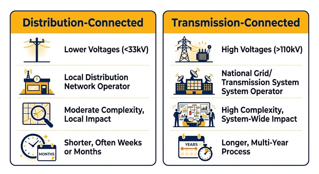
The first choice point in the BESS interconnection process is the connection voltage: distribution or transmission.
Distribution-Connected BESS
This path fits most C&I and smaller utility projects.
- Connects directly to medium- or low-voltage distribution networks.
- Managed by the local distribution utility or DSO/DNO as the interconnection authority.
- Features a standardized, streamlined pathway with screening for smaller systems.
- Grid-code requirements also cover ride-through, frequency response, reactive-power support, protection, and power quality.
Because rules vary by country, see our BESS grid codes and compliance guide for the specifics.
Transmission-Connected BESS
This path fits large utility-scale plants.
- Connects to high-voltage transmission networks.
- Also, the TSO, ISO/RTO, or transmission owner is the interconnection authority.
- The process also involves multiple study phases, detailed modeling, and often significant network upgrades.
- Grid-code requirements are stricter too, covering fault-ride-through, frequency response, fault-current, and modeling obligations.
As a result, transmission projects often face longer queues and closer coordination between the TSO, owner, and any off-takers.
The BESS Interconnection Process: Step by Step
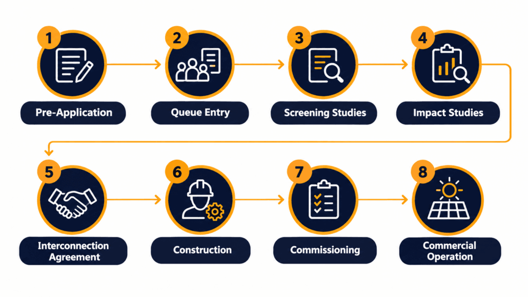
Most projects move through the same broad BESS interconnection process, even though the details vary by market.
Step 1: Pre-Application and Feasibility
Before filing, developers confirm the point of interconnection and connection voltage.
- First, confirm the applicable system operator, distributor, and interconnection rules.
- Next, prepare a preliminary single-line diagram, equipment list, and control architecture.
- Then, run feasibility studies to screen for thermal overloads, voltage issues, or protection conflicts.
Because of that, early engagement with the utility or TSO clarifies queue status and likely upgrade needs.
Point of interconnection (POI) vs. point of common coupling (PCC): the POI is where the project connects to the utility or transmission network. The PCC is the electrical point shared with other network users. Depending on project layout, the POI and PCC may be at the exact same location or separated by short network distances.
Step 2: Interconnection Request and Queue Entry
The formal BESS interconnection process usually starts with a written application.
- For example, project details include capacity, technology, expected in-service date, and point of interconnection.
- It also includes technical data: inverter models, ride-through behavior, protection settings, and control modes.
- Finally, it includes an application fee and a queue position.
The project then waits in a queue for studies to begin, and queue position can affect cost allocation.
Step 3: Screening and Scoping Studies
Distribution projects usually start with a screening study.
- First, it checks basic compliance with the distribution code.
- It also flags overloads, voltage violations, or protection conflicts.
- As a result, it can lead to fast-track approval for small, compliant systems.
Transmission projects instead run a scoping study or cluster screen.
- First, it defines which studies are required: impact, facilities, or system impact.
- Then, it sets the models and data the developer must supply.
- Finally, it flags preliminary upgrade candidates and cost responsibility.
Step 4: Impact and System Studies
This is the core technical phase of the BESS interconnection process, especially for transmission-connected BESS.
- Short-circuit and fault-level studies verify protection coordination and fault-current contributions.
- Also, voltage and thermal studies check steady-state and dynamic voltage profiles and equipment loading.
- In turn, protection coordination studies align BESS protection with utility or TSO schemes and ride-through rules.
- Stability and dynamic-performance studies also assess frequency response and interaction with other resources.
- Meanwhile, harmonic and power-quality studies confirm limits on harmonics, flicker, and DC injection.
- System-strength, control-interaction, or electromagnetic-transient studies, where required, check whether inverter controls stay stable in weak-grid conditions and interact properly with nearby inverter-based resources.
For a closer look at how each of these studies actually works — load flow, short-circuit, protection coordination, harmonics, and RMS/EMT modelling — see our BESS grid connection studies guide.
As a result, the output is a system impact report listing required upgrades, protection changes, and any operating constraints.
Step 5: Interconnection Agreement and Project Milestones
Once the required studies are complete, the developer and the relevant utility, transmission provider, system operator, or network operator negotiate and execute an interconnection agreement or equivalent connection agreement.
- First, it sets technical requirements: ride-through curves, frequency response, reactive-power capability, and protection settings.
- It also covers network upgrades: who designs, builds, and pays for each one.
- Then it sets milestones: financial security, construction start, substantial completion, and commercial operation date.
- Finally, it defines testing and compliance requirements: model validation, commissioning tests, and ongoing reporting.
In turn, signing the agreement usually triggers financial security postings and a firmer construction schedule.
Step 6: Construction and Equipment Installation
During this stage of the BESS interconnection process, the owner and EPC install the physical plant.
- This includes battery containers, PCS, transformers, switchgear, and protection systems.
- It also covers the control architecture: plant controller, SCADA, communications, and telemetry.
- Throughout, the team coordinates with the utility or TSO on any network upgrades or substation work.
As a result, good documentation and early coordination reduce delays at commissioning.
Step 7: Commissioning and Compliance Testing
Before moving to commercial operation in the BESS interconnection process, the plant must prove compliance with the interconnection agreement.
- For example, ride-through and frequency-response verification covers LVRT/HVRT, frequency ride-through, and control behavior, demonstrated through the method the operator requires — site measurements, controller records, model validation, staged tests, or another approved procedure.
- It also runs frequency-response tests: droop, deadband, and response time.
- Then come reactive-power and voltage-control tests: fixed Q/V, droop, and power-factor capability.
- Protection tests follow too: over/under voltage and frequency, overcurrent, earth fault, and anti-islanding.
- So do power-quality tests: harmonics, flicker, unbalance, and DC injection.
- Finally, model validation compares simulated and measured responses.
Together, successful commissioning tests, completed documentation, and required inspections fulfill the technical criteria. Once network-upgrade and telemetry obligations are confirmed, the system operator can grant final permission to operate or authorize commercial operation.
Step 8: Commercial Operation and Ongoing Compliance
Once the BESS interconnection process is complete, the project officially enters commercial operation.
- First, it maintains compliance with grid-code settings and protection.
- It also provides telemetry, performance data, and availability reports to the system or market operator.
- In addition, it participates in required markets or programs: capacity, ancillary services, or flexibility.
- Finally, it manages changes: equipment or control updates may trigger re-approval or new studies.
Otherwise, non-compliance can bring penalties, export limits, or mandatory corrective action.
How Grid Codes Shape the BESS Interconnection Process
Grid codes are not a side checkbox. Instead, they drive most of the BESS interconnection process.
- First, study inputs: ride-through curves, frequency-response parameters, and reactive-power capability feed the impact and stability studies. See our BESS grid codes and compliance guide.
- Also, equipment selection: inverter and PCS capability must match the applicable code. See our BESS PCS functions and features guide and Understanding BESS specifications guide.
- In turn, testing scope: commissioning tests verify ride-through, frequency response, reactive power, protection, and power quality directly. See our LVRT and HVRT guide and Fast Frequency Response (FFR) guide.
- Finally, market participation: many capacity and ancillary-service products require proof of specific grid-code performance. See our BESS revenue streams and value-stacking guide.
Together, a well-coordinated strategy lines up grid-code compliance, equipment selection, and market plans from day one.
Typical Timelines and Cost Drivers in the BESS Interconnection Process
However, timelines and costs vary widely by market, project size, and network conditions.
Distribution-Connected BESS Timeline
Smaller systems often connect within months, assuming no major upgrades.
- For example, cost drivers include application and study fees, minor protection or transformer upgrades, and local voltage support.
- Risk factors also include feeder constraints, high DER penetration, and conservative utility practices.
Transmission-Connected BESS Interconnection Process Timeline
Large plants often take years from application to commercial operation, especially in congested queues.
- Cost drivers include network upgrades, extended studies, financial security, and prolonged commissioning.
- Risk factors also include queue position, cluster effects, and evolving grid-code or market requirements.
For how these factors affect project economics, see our BESS CAPEX calculation and OPEX model.
Practical Tips to De-Risk the BESS Interconnection Process
A consistent approach to the BESS interconnection process helps teams developing multiple projects.
- First, engage early: talk to the utility or TSO before filing to learn queue status and likely constraints.
- Second, design for compliance: pick inverters and PCS with proven ride-through, frequency-response, and protection capability.
- Third, invest in good models: accurate plant models cut study iterations and commissioning surprises.
- Fourth, plan for testing: budget time and cost for ride-through, frequency, reactive-power, protection, and power-quality tests.
- Finally, document changes: track any equipment or control change during construction and re-approve where required.
Together, our BESS grid codes and compliance guide and Understanding BESS specifications guide can help translate these requirements into concrete equipment and control specifications.
Frequently Asked Questions
These common questions cover the BESS interconnection process in more detail.
What Is the BESS Interconnection Process?
In short, the BESS interconnection process is the set of steps a battery storage project completes to connect to the grid and start commercial operation.
It includes the application, technical studies, grid-code compliance, construction, commissioning tests, and final approval.
Also, distribution-connected projects often have a more standardized, potentially faster pathway than transmission-connected plants, particularly when no major feeder or transformer upgrades are needed.
How Long Does the BESS Interconnection Process Take?
Timing depends on project size, connection voltage, location, queue rules, study complexity, and required network upgrades.
For example, smaller distribution-connected BESS projects may complete interconnection in months when the local network has capacity and no major upgrades are needed.
Transmission-connected projects can take years because of queue backlogs, cluster studies, network upgrades, financial-security milestones, detailed modeling, and commissioning requirements.
What Studies Are Required for BESS Interconnection?
Common studies include short-circuit and fault-level, voltage and thermal, protection coordination, stability and dynamic-performance, and harmonic and power-quality studies.
In general, transmission projects typically need more extensive studies and detailed modeling than distribution projects.
Do C&I Projects Follow the Same BESS Interconnection Process as Utility-Scale?
The basic steps are similar, but the detail differs.
For example, C&I and distribution-connected projects usually follow a standardized process with screening and simplified studies.
By contrast, utility-scale and transmission-connected BESS face more complex studies, stricter grid codes, and longer timelines.
What Happens if a BESS Fails Interconnection Tests?
If a BESS fails commissioning or grid-code tests, the network operator may delay permission to operate, require hardware, firmware, protection, or control changes, or restrict export capacity.
The developer may also need to repeat studies or validation tests if the final installed equipment differs from the approved models.
So, permission to operate is normally granted only after corrective actions, documentation, and required verification are complete.
Further Reading
These related guides cover topics referenced throughout this BESS interconnection process overview.
- BESS Grid Codes and Compliance: Global Requirements by Country
- LVRT and HVRT: Voltage Ride-Through for BESS and Solar
- Fault Ride-Through Features in PCS Hardware & Control
- Fast Frequency Response (FFR)
- BESS PCS Functions and Features
- Understanding BESS Specifications
- BESS CAPEX Calculation
- BESS OPEX and Operating Cost Model
- Cost of Storing Energy: BESS LCOS Calculator Guide
- BESS Revenue Streams and Value Stacking
- ESS Codes and Standards for USA Utility-Scale BESS
- U.S. Department of Energy – Interconnection Innovation e-Xchange (i2X)

BESS Grid Codes and Compliance: Global Rules by Country
BESS grid codes are the technical interconnection requirements a battery storage project must meet to connect to and operate on the grid. They cover voltage and frequency ride-through, reactive-power support, protection coordination, power quality, testing, and compliance documentation. Getting these BESS interconnection requirements right affects approval speed, project cost, and long-term revenue.
Quick Answer: BESS grid codes are the technical interconnection requirements battery storage projects must meet to connect and operate on the grid. They cover voltage and frequency ride-through, reactive-power capability, protection coordination, power quality, testing, and compliance documentation. Standards vary by market: IEEE 1547 and IEEE 2800 in the US, ENTSO-E RfG and national codes in the EU, G99 in the UK, and NER, AEMO, TNSP, and DNSP requirements in Australia.
Why BESS Grid Codes Matter for Storage Projects
Grid codes exist to keep the power system stable as more inverter-based resources connect. For BESS, three practical outcomes are at stake.
- Connection approval: a non-compliant design can be rejected or delayed at the study or commissioning stage.
- Market participation: many capacity, ancillary-service, and flexibility products require proof of compliance with a specific grid code.
- Cost and risk: compliance shapes inverter selection, protection design, studies, testing, and sometimes CAPEX and OPEX.
For the cost side of compliance, see our BESS CAPEX calculation and BESS OPEX model guides. Our BESS revenue streams and value-stacking guide covers how compliant performance turns into income. For the project workflow that turns these technical requirements into an approved grid connection—from application and studies through commissioning and commercial operation—see our BESS interconnection process guide.
Core Technical Rules in BESS Grid Codes
Details vary by market. Even so, most modern grid codes expect the same core capabilities from a BESS.
Voltage Ride-Through: LVRT and HVRT

Low Voltage Ride Through (LVRT) and High Voltage Ride Through (HVRT) require inverters to stay connected during short voltage sags and swells, rather than tripping offline. Under LVRT, a BESS may need to stay connected through a defined voltage dip for a specified duration and provide reactive-current support.
Under HVRT, it may need to tolerate a defined overvoltage event and absorb or adjust reactive power. Exact voltage-versus-time curves and current-response rules depend on specific BESS grid codes, connection voltage, and project interconnection agreements, so treat any single number as illustrative, not universal. In the US, IEEE 1547-2018 governs distribution-connected systems, and IEEE 2800-2022 governs transmission-connected plants. For the detailed curves and numbers, see our LVRT and HVRT guide.
A compliant curve on a datasheet only states the target. Our Fault Ride-Through Features guide goes a level deeper into the PCS hardware and control functions, like current limiting and DC-link protection, that actually make a unit meet that curve.
Frequency Ride-Through and Fast Frequency Response
Frequency ride-through is another core piece of most BESS grid codes: it requires a BESS to stay connected during under- and over-frequency events. Many markets also expect fast frequency response (FFR), a rapid active-power change in response to a frequency deviation.
- Defined under-frequency and over-frequency trip thresholds and delays
- Frequency-droop control, and synthetic-inertia-like behavior in some markets
- Testing through simulation or field tests during commissioning
See our Fast Frequency Response (FFR) guide for how this works in practice.
Reactive Power and Power Factor
Most grid codes require a BESS to provide reactive power support and to hold a specified power-factor range. Common rules include leading and lagging operation, for example 0.95 leading to 0.95 lagging, plus fixed-Q, fixed-V, or droop voltage-control modes.
These capabilities shape inverter sizing, transformer design, and plant-controller logic. Our BESS power factor guide covers the underlying reactive-power mechanics in more depth.
Protection and Power Quality
In addition to ride-through rules, BESS grid codes set strict protection and power-quality expectations.
- Over/under voltage and over/under frequency protection settings aligned with ride-through duties
- Overcurrent, earth-fault, and sometimes differential protection
- Limits on harmonics, DC injection, flicker, and unbalance
- Anti-islanding and run-on rules for distribution-connected systems
Protection must be coordinated from the inverter through the AC collection system to the point of common coupling, while still meeting ride-through obligations.
How BESS Grid Codes Are Verified: Approval and Testing
Compliance with BESS grid codes is shown through a mix of product approval and project-level testing.
Product Certification and Type Approval
In many markets, inverters and sometimes complete BESS packages need approval to recognized standards.
- In the US and Canada, UL 1741 certification, together with the applicable supplement and IEEE 1547.1 test procedures, is commonly used to demonstrate inverter safety and grid-interactive functionality
- IEC 62109, covering power-conversion equipment safety
- Regional type approval or conformity marks, such as CE in Europe, with the exact pathway depending on system size and connection voltage
Approval shows the equipment can meet basic grid-code functions in a controlled test environment, not that a specific project is automatically compliant.
Plant-Level Studies and Commissioning Tests
For utility-scale and many C&I projects, the system operator or distributor also requires plant-level verification.
- Connection studies covering short-circuit, protection coordination, and voltage impact
- Model quality testing, to confirm simulation models match measured plant behavior
- Commissioning tests for ride-through, frequency response, protection, and power quality at the point of common coupling
See our BESS grid connection studies guide for how each of these studies — load flow, short-circuit, protection coordination, harmonics, and RMS/EMT modelling — actually works.
Together, these confirm that the combined response of every inverter and the plant controller meets the applicable grid code.
BESS Grid Codes by Country and Region

The sections below summarize how major markets approach BESS grid codes. Exact rules depend on connection voltage, project size, and the specific system operator or distributor.
Important: this guide is a planning overview, not a substitute for a project’s applicable interconnection agreement. Requirements can differ by project capacity, connection voltage, location, network operator, technology configuration, and commissioning date. The table below is a high-level orientation tool — always verify project-specific rules with the relevant network operator.
| Market | Primary framework | Typical BESS focus | Project-level authority |
| United States | IEEE 1547-2018; IEEE 2800-2022; UL 1741 | Ride-through, reactive support, protection, modeling | Utility, ISO/RTO, transmission owner |
| European Union | ENTSO-E RfG plus national codes | Fault current, FRT, frequency support, testing | TSO/DSO and national rules |
| United Kingdom | G99 and network-operator requirements | FRT, reactive power, dynamic testing | DNO/DSO and relevant network operator |
| Australia | NER, AEMO, TNSP/DNSP requirements | System strength, voltage/frequency response, protection | AEMO, TNSP, DNSP |
| India | CEA rules, Grid-India, state requirements | Evolving FRT, reactive support, connection | SLDC, DISCOM, transmission utility |
United States
US grid codes come mainly from IEEE 1547-2018 for distribution-connected systems and IEEE 2800-2022 for transmission-connected plants. UL 1741, together with the applicable supplement and IEEE 1547.1 test procedures, is commonly used to demonstrate inverter compliance, including ride-through behavior, and regional ISOs and RTOs such as CAISO, ERCOT, PJM, and NYISO add market-specific rules.
IEEE 1547 sets voltage and frequency ride-through categories, reactive-current support, and anti-islanding. IEEE 2800 raises the bar further for transmission plants, with stricter ride-through, fault-current, and modeling rules. Compliance affects both connection approval and eligibility for capacity and ancillary-service markets. For the USA fire, electrical, and product-safety side of compliance, separate from grid-connection rules, see our ESS codes and standards guide.
European Union
European BESS grid codes sit under the ENTSO-E Requirements for Generators (RfG) framework, which sets high-level rules for every generator type, including storage. National codes then implement the detail. These can differ materially from US requirements, particularly when comparing project connection voltage, plant size, and the applicable IEEE 1547 or IEEE 2800 framework.
Germany applies VDE-AR-N 4110 and 4120 for medium- and high-voltage connections. Spain, Italy, and the Nordic countries follow RfG with local variations in curves and testing. Developers should always confirm the national code and the TSO or DNO rules for the specific connection point.
United Kingdom
UK grid codes take the form of the country’s own connection rules for generation and storage. These were historically influenced by the EU Requirements for Generators framework, but since Brexit, projects are governed through UK-specific rules such as Engineering Recommendation G99 and the requirements of the relevant network operator.
G99 defines fault-ride-through profiles, reactive-power rules, and dynamic-performance tests, and often calls for detailed modeling and commissioning tests to verify compliance.
Australia
Australian grid codes work differently for each connection level. Transmission-connected BESS projects are governed primarily by the National Electricity Rules (NER), AEMO requirements, and the applicable transmission network service provider’s connection process. Distribution-connected BESS projects must meet the relevant Distribution Network Service Provider (DNSP) connection requirements, including voltage, frequency, protection, and ride-through settings.
DNSPs set project-specific connection settings for distribution-connected BESS. These can include voltage and frequency disturbance ride-through, reactive-power control, export limits, protection settings, and inverter-response modes, and both the terminology and the settings vary by DNSP and state.
For many distribution-connected systems, Clean Energy Council (CEC) listing and DNSP-approved inverter settings may be relevant; the exact approval pathway depends on system size, state, connection voltage, and the local DNSP. System strength or fault-level issues in some regions can also affect inverter selection. Compliance determines eligibility for FCAS and other markets, so early engagement with the DNSP and AEMO matters for C&I and utility projects.
India
Grid-code rules for storage are still evolving alongside renewable and hybrid projects. Central Electricity Authority (CEA) regulations and Grid-India rules set high-level standards, while state load dispatch centers and distribution companies apply connection rules that vary by state.
LVRT/HVRT, frequency ride-through, and reactive-power support are increasingly expected for larger projects at transmission and sub-transmission level. Developers should confirm the latest rules with the relevant SLDC and state agency, since rules for standalone BESS are still maturing.
Other Markets
Other markets set their own grid codes but follow a similar pattern. Canadian provinces apply ride-through and protection rules often aligned with IEEE and UL standards. Japan and Korea set fault-ride-through and frequency rules through national utilities and standards bodies, and Middle East markets such as Saudi Arabia and the UAE reference international standards with local amendments.
In every case, the same principle applies: ride through faults, support voltage and frequency, meet protection and power-quality standards, and prove compliance through approval and testing.
How BESS Grid Codes Affect Project Economics
Grid-code compliance is not only a technical checkbox. It shapes project economics in four ways.
- CAPEX: stricter ride-through, fault-current, and protection rules can drive inverter selection, transformer sizing, and protection equipment cost
- OPEX: added testing, monitoring, and maintenance to stay compliant can raise operating cost
- Revenue and risk: compliance decides whether a BESS can join capacity, ancillary-service, or flexibility markets, and avoid non-performance penalties
- LCOS: all of the above feed into the lifetime cost of stored energy
See our BESS CAPEX calculation, BESS OPEX model, and LCOS calculator guide for the cost side, and our BESS revenue streams and value-stacking guide for the market side. A technically compliant design that ignores cost and revenue can still be a weak investment case.
Practical Steps for BESS Grid Code Compliance
Teams developing BESS projects across multiple markets benefit from a consistent process.
Start with the project’s interconnection agreement and the network operator’s technical schedule. National standards and certification documents support compliance, but the project-specific agreement controls the final requirements.
- Identify the applicable grid code early, and confirm whether the project connects at distribution or transmission level
- Map rules to inverter and PCS capabilities, including LVRT/HVRT curves, frequency ride-through, reactive power, protection, and approval
- Engage the system operator or distributor early to clarify study and modeling expectations
- Budget time and cost for product approval, model validation, and commissioning tests
- For multi-market designs, build to the strictest common requirement, then adapt settings per market
Our BESS PCS functions and features guide and Understanding BESS Specifications guide help translate these rules into a concrete equipment specification.
Frequently Asked Questions
Common questions readers ask about BESS grid codes, answered directly.
What Are BESS Grid Codes?
BESS grid codes are the technical rules system operators and regulators set for connecting battery storage to the grid. They cover fault behavior (LVRT/HVRT, frequency ride-through), voltage and frequency support, and required approval and tests. Rules vary by country and by connection voltage.
Which Standards Define BESS Grid Codes in the US?
US grid codes rest mainly on IEEE 1547-2018, which covers most distribution-connected DER, and IEEE 2800-2022, which applies to transmission-connected inverter-based resources. IEEE 1547.1 defines test procedures for DER connection functions. In the US and Canada, UL 1741 certification, together with the applicable supplement, test procedure, and local utility requirements, is commonly used to demonstrate inverter safety and grid-interactive functionality. ISOs, RTOs, transmission owners, and utilities may add further connection, telemetry, modeling, or market-participation rules.
How Do EU Grid Codes for BESS Differ From the US?
EU grid codes sit under the ENTSO-E Requirements for Generators (RfG) framework, which sets EU-wide rules, and national codes such as Germany’s VDE-AR-N 4110/4120 add local detail. These often specify detailed fault-current, ride-through, and dynamic-performance rules that can differ materially from US requirements, particularly when comparing connection voltage, plant size, and the applicable IEEE 1547 or IEEE 2800 framework. The UK, no longer an EU member, follows its own G99 framework with similar technical goals.
Do BESS Grid Codes Apply to C&I Projects as Well as Utility-Scale?
Yes, though the detail differs. Utility-scale and transmission-connected BESS face the strictest grid codes. C&I and distribution-connected projects still must meet the applicable distribution code, such as IEEE 1547 in the US, G99 in the UK, or the relevant DNSP’s connection requirements in Australia.
What Happens if a BESS Project Does Not Meet Grid-Code Rules?
If a project cannot show it meets the applicable grid codes, the system operator or distributor can refuse permission to operate, require hardware or control changes, or cap the plant’s export capacity. In practice, this can mean reprogramming inverters, adjusting plant controllers, or revising protection settings before the project can energize.
Further Reading
More Sunlith Energy guides related to BESS grid codes and interconnection compliance.
- LVRT and HVRT: Voltage Ride-Through for BESS and Solar
- Fault Ride-Through Features in PCS Hardware & Control
- Fast Frequency Response (FFR)
- BESS PCS Functions and Features
- Understanding BESS Specifications
- BESS CAPEX Calculation
- BESS OPEX and Operating Cost Model
- Cost of Storing Energy: BESS LCOS Calculator Guide
- BESS Revenue Streams and Value Stacking
- ESS Codes and Standards for USA Utility-Scale BESS
- BESS Power Factor Explained
- U.S. Department of Energy, Office of Electricity: Energy Storage
BESS Revenue Streams and Value Stacking: How Storage Projects Make Money
A BESS rarely makes money from a single source. Most viable projects combine several BESS revenue streams.
For instance, these typically include energy arbitrage, capacity payments, ancillary services, demand-charge reduction, backup power, and sometimes local flexibility or network-support contracts.
So value stacking is the practice of combining these streams so they improve project economics, without overcommitting the asset.
Quick Answer: BESS revenue streams include energy arbitrage, capacity payments, ancillary services, demand-charge savings, backup power value, and local flexibility or network-support contracts. Value stacking combines multiple streams on the same asset to improve returns, while respecting technical limits and contract constraints.
In this guide, “value” includes both direct revenue, such as market payments, and avoided costs, such as demand-charge reduction, lower energy purchases, and avoided outage losses.
Why Value Stacking Matters for BESS Revenue Streams
A battery has limited energy and power. If you use it for only one service, you may leave value on the table.
For example, a system sized for demand-charge management may sit idle for large parts of the day. That idle time could support arbitrage, frequency response, or other services instead.
Value stacking aims to:
- Increase total annual revenue and savings
- Improve utilization of the same CAPEX investment
- Diversify revenue risk across multiple products or tariff mechanisms
- Support grid services while meeting customer needs
But stacking also adds complexity. Each revenue stream carries its own operating profile, performance requirements, and sometimes conflicting dispatch needs.
Because of this, a robust revenue model must respect energy availability, power limits, degradation impacts, and contract obligations.
For context on how revenue and savings interact with costs, see our CAPEX vs LCOS guide, our BESS OPEX model, and our LCOS calculator guide.
Common BESS Revenue Streams
The available revenue streams depend on market rules and tariff design. They also depend on whether the BESS sits in front of the meter or behind it.
Energy Arbitrage
Energy arbitrage buys cheap electricity and sells it when prices rise. For example, in wholesale markets, that usually means charging during low-price periods and discharging during peak-price periods.
But in tariff-based environments, it instead means shifting load from high-price time-of-use blocks to lower-price blocks. Key drivers include:
- Price spread between low and high price periods
- Duration and depth of price peaks
- Round-trip efficiency and losses
- Cycling frequency and degradation impact
Arbitrage often anchors revenue for utility-scale BESS, but it also plays an important role for C&I projects on time-of-use rates.
Capacity Payments and Resource Adequacy
Many markets pay for available capacity, not just energy. So a BESS may earn capacity payments for qualifying and remaining available to discharge during defined peak or reliability periods.
For example, eligibility commonly depends on market rules, duration, testing, availability commitments, and performance requirements.
- Payments usually run in dollars per kW-year or dollars per kW-month
- Availability and performance requirements can be strict
- Duration requirements, such as 2-hour or 4-hour, affect eligibility and value
- Capacity value can be a major revenue component in resource-adequacy markets
Capacity revenue often pairs well with arbitrage. For example, the battery may cycle for price spreads while still holding enough reserved energy to meet capacity obligations.
Ancillary Services and Frequency Regulation
Ancillary services include frequency regulation, spinning and non-spinning reserves, voltage support, and black-start capability. Frequency regulation suits batteries well, because they respond fast and control output precisely.
- In some markets, can offer higher value per MW than energy arbitrage, though pricing, saturation risk, and qualification rules vary significantly by market and over time
- Requires fast response, high availability, and accurate tracking
- May involve many small cycles, which affects degradation
- Market rules and qualification criteria vary by region
In some early-stage or fast-response markets, ancillary services can be a major BESS revenue source. As participation increases, service prices and available volumes may decline, so models should not assume historic revenues persist unchanged.
Demand-Charge Reduction (Behind-the-Meter)
For commercial and industrial customers, demand charges can make up a large share of the electricity bill. So a BESS can lower that charge by discharging during peak intervals.
- Savings depend on tariff structure and peak demand profile
- Often ranks among the most valuable C&I use cases
- Requires accurate peak prediction and control logic
- Can combine with solar PV to maximize self-consumption and peak shaving
Demand-charge reduction counts as revenue in the sense of avoided cost, because it lowers a bill the customer would otherwise pay. It frequently anchors the business case for C&I BESS.
Backup Power and Resilience Value
A BESS can supply backup power during outages and support critical loads. This carries value even when no market directly pays for it:
- Avoided production losses or downtime costs
- Improved safety and continuity for critical facilities
- Avoided spoilage, unplanned restart cost, data loss, or contractual penalties
- Explicit resilience incentives or payments, in some programs
Resilience value is commonly estimated from avoided outage cost. However, whether these benefits can be treated as quantified project value depends on the facility’s outage history, critical-load profile, and internal risk methodology.
Local Flexibility, Network Support, and Non-Wires Alternatives
Utilities and system operators increasingly use storage as part of local flexibility or non-wires solutions. A BESS may earn payments or contracts for:
- Deferring distribution or transmission upgrades
- Managing local congestion or voltage issues
- Providing targeted support during outages or peak events
- Participating in flexibility markets or pilot programs
These contracts are often project-specific, but they can add significant value in constrained networks.
Renewable Integration and Self-Consumption Optimization
When paired with solar or wind, a BESS can:
- Increase self-consumption of on-site generation
- Shift renewable output to higher-value periods
- Reduce curtailment and improve project economics
- Support compliance with renewable or storage mandates
This matters most for C&I solar-plus-storage projects and utility-scale hybrid plants. So a solar-plus-storage system can shift midday solar output into the evening peak.
How BESS Revenue Streams Combine in Value Stacking

Value stacking is not simply adding up every possible revenue stream. Because the battery has limits, a realistic model has to weigh several factors together.
- Energy and power limits: the battery can’t commit the same kWh or kW to multiple services at once
- Dispatch priority: some services, like frequency regulation or capacity obligations, may outrank others
- Degradation impact: heavier cycling and deeper depth of discharge can speed up degradation, which affects long-term revenue and LCOS
- Contract and market rules: some programs restrict participation in other markets or require minimum availability
- Forecast uncertainty: because price, load, and renewable output are all uncertain, robust strategies lean on scenarios and risk management
A simple conceptual model sums revenue and savings across streams:
Total Annual Value = Σi Revenuei + Σj Savingsj
Here, i indexes market revenue streams, such as arbitrage, capacity, ancillary services, and flexibility contracts. j indexes savings streams, such as demand-charge reduction, backup and resilience, and increased self-consumption.
So the optimization problem then allocates available energy and power across these streams over time. The goal is to maximize net present value or IRR, subject to technical and contractual constraints.
Example Dispatch Hierarchy
Example dispatch hierarchy for a C&I BESS: A facility may reserve 1 MW of discharge power and 1.2 MWh of usable energy for forecasted monthly demand peaks. Outside the forecast peak window, the energy-management system may use unreserved capacity for TOU optimization or eligible flexibility events. If an outage-resilience commitment applies, the minimum backup state of charge overrides both economic dispatch opportunities.
This kind of hierarchy is why value stacking can’t simply add every stream together. So each layer has to respect what the layer above it already reserved.
From Gross Value to Net Project Value
That distinction also matters when you move from gross value to project economics.
Net Annual Project Value = Gross Revenue and Savings −
Operating Cost − Degradation/Replacement Allowance
Use net annual project value, not gross revenue alone, when you assess payback, NPV, IRR, or the viability of a proposed value stack. Pull Operating Cost from your BESS OPEX model, and the degradation/replacement allowance from your LCOS guide.
Simple BESS Revenue Streams Example: 2 MWh C&I System
Consider a 2 MWh, 1 MW C&I BESS with simplified annual value streams.
Demand-charge savings come from a peak demand reduction of 400 kW, at a demand charge of $15 per kW-month.
Annual savings: 400 × $15 × 12 = $72,000
Energy arbitrage, or TOU optimization, brings a net annual benefit from shifting 500 MWh from high-price to low-price periods. The average price spread runs $20 per MWh.
Annual arbitrage value: 500 × $20 = $10,000
A capacity or local flexibility payment recognizes 500 kW for capacity or local support, at $30 per kW-year.
Annual revenue: 500 × $30 = $15,000
Backup and resilience value stays qualitative here. It covers avoided downtime and continuity benefits, but this example doesn’t monetize it directly.
| Value Stream | Basis | Annual Value |
| Demand-charge savings | 400 kW × $15/kW-month × 12 | $72,000 |
| Energy arbitrage / TOU | 500 MWh × $20/MWh spread | $10,000 |
| Capacity / local flexibility | 500 kW × $30/kW-year | $15,000 |
| Total quantified value | Before OPEX and degradation | $97,000/year |
Avoiding Double-Counting in the Value Stack
Important: The $97,000 total assumes these services occur in compatible time windows and do not claim the same battery power or energy at the same time. In a real dispatch model, reserve the required state of charge and power capacity for priority services before assigning remaining capability to arbitrage or flexibility opportunities.
If a capacity or local-flexibility contract requires the battery to remain available during the same peak period used for demand-charge reduction, the model must assign a dispatch priority. Otherwise, it must reduce one of the two value assumptions.
From Example to Full Financial Model
In a full model, you would take a few more steps. First, subtract annual OPEX using your BESS OPEX model.
Then account for degradation and any augmentation or replacement CAPEX. Next, discount cash flows to compute NPV and IRR.
Finally, compare the result to CAPEX from your BESS CAPEX calculation and LCOS from your LCOS guide.
This example is illustrative only. So actual values depend on tariff design, load profile, market rules, and system design.
Front-of-the-Meter vs Behind-the-Meter BESS Revenue Streams
Revenue opportunities differ by project type.
Front-of-the-meter projects, meaning utility or wholesale assets, typically access:
- Energy arbitrage in wholesale markets
- Capacity payments and resource adequacy
- Ancillary services, such as frequency regulation and reserves
- Local flexibility or network-support contracts
- Renewable integration in hybrid plants
Key constraints here include market qualification and performance requirements, competition from other resources, and transmission or interconnection limits.
Behind-the-meter projects, such as C&I, commercial, and community systems, typically access:
- Demand-charge reduction
- TOU optimization and self-consumption
- Backup power and resilience
- Participation in demand-response or flexibility programs, where available
- Possible capacity or local-support payments, depending on the market
Key constraints here include customer load profile and tariff structure. Interconnection and export limits also matter, along with customer priorities like resilience versus revenue maximization.
Because of this split, many C&I projects lean primarily on demand-charge savings and resilience. Arbitrage and program participation add incremental value on top.
Risks and Limitations of Value Stacking
Value stacking improves economics, but it also introduces risks:
- Over-commitment: committing the same capacity to multiple services can cause shortfalls and penalties
- Revenue cannibalization: some streams compete for the same energy at the same time
- Degradation acceleration: more intensive use can speed up degradation, raising LCOS and reducing long-term value
- Market and policy risk: rules, prices, and program availability can change
- Operational complexity: more streams demand more sophisticated control, forecasting, and monitoring
A conservative approach works better for most projects. So prioritize a few core streams with clear value and manageable risk.
Then leave headroom for uncertainty and degradation, and reassess your stacking strategy as markets and tariffs evolve.
Frequently Asked Questions
What Is the Most Important BESS Revenue Stream?
It depends on the market and project type. However, for utility-scale BESS, capacity payments and ancillary services often matter most, alongside arbitrage.
For C&I BESS, demand-charge reduction and resilience usually drive the primary value, with arbitrage and program participation adding secondary value.
Can a BESS Rely on a Single Revenue Stream?
Some projects do, especially in markets with strong capacity or ancillary-service value. However, most bankable business cases rely on multiple streams, because that diversifies risk and improves asset utilization.
How Do I Avoid Over-Stacking a BESS?
Use a dispatch and optimization model that respects energy and power limits, availability requirements, and degradation impacts.
Start with conservative assumptions. Then refine them as you gain operational data and market experience.
Further Reading
- BESS CAPEX Calculation: How to Build the Total Investment Cost
- CAPEX vs LCOS: What BESS Cost per kWh Really Means
- Cost of Storing Energy: BESS LCOS Calculator Guide
- BESS OPEX and Operating Cost Model: What Really Drives Annual Expenses
- The Economics of BESS: Calculate ROI for Your Energy Storage
- Understanding BESS Specifications: The Complete 2026 Guide
- U.S. Department of Energy, Office of Electricity: energy storage program overview